

Key processing steps that have been improved in the V3 data release are shown in bold in the flow diagram in the blue box. Italics show interim values calculated during the stepwise process.
The movie at right compares data processed using Version 2 (V2) and V3 algorithms. Maps are from September 2011, the first full month during which Aquarius salinity data were collected. The movie begins by transitioning from V2 to V3 data on a global map, followed by a V2-to-V3 transition focused on an area in the eastern equatorial Pacific Ocean. Orange colors depict relatively high salinity (> 37) while dark blues show relatively low salinity areas (< 33).
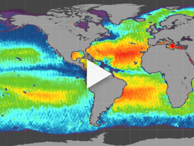
The movie above compares data processed using Version 2 (V2) and V3 algorithms. Maps are from September 2011, the first full month during which Aquarius salinity data were collected. The movie begins by transitioning from V2 to V3 data on a global map, followed by a V2-to-V3 transition focused on an area in the eastern equatorial Pacific Ocean. Orange colors depict relatively high salinity (> 37) while dark blues show relatively low salinity areas (< 33).
Reflection of the galaxy on the ocean surface has a big impact on the quality of Aquarius' salinity data. This became clear when comparing V2 data collected over the same area when the satellite was ascending versus descending in its orbit. Why? The Aquarius pointing geometry was tilted (i.e., not pointing straight down) and the ocean surface can act like a mirror. Depending on which direction the satellite is moving, galactic radiation can be reflected toward or away from the instrument.
The movie at left illustrates where Aquarius data were acquired (i.e., green ovals) relative to its orbital path. It begins with the satellite descending on the visible side of Earth. Next, ascending orbits crossed near the north pole and descended on the opposite side. Finally, it shows where ascending and descending swaths overlapped. Comparing data from these areas of overlap helped to understand how to correct for galactic reflection off the ocean surface.
The movie above illustrates where Aquarius data were acquired (i.e., green ovals) relative to its orbital path. It begins with the satellite descending on the visible side of Earth. Next, ascending orbits crossed near the north pole and descended on the opposite side. Finally, it shows where ascending and descending swaths overlapped. Comparing data from these areas of overlap helped to understand how to correct for galactic reflection off the ocean surface.
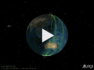
Figure 1 illustrates where Aquarius data were acquired (i.e., green ovals) relative to its orbital path. It begins with the satellite descending on the visible side of Earth. Next, ascending orbits crossed near the north pole and descended on the opposite side. Finally, it shows where ascending and descending swaths overlapped. Comparing data from these areas of overlap helped to understand how to correct for galactic reflection off the ocean surface.
Examining V2 ascending versus descending data resulted in a more accurate "Geometric Optics" (GO) model for V3, which takes into account orbit position (y-axis in the graph at left - click to enlarge) versus month (x-axis). Red values are equivalent to corrections of 6 practical salinity units, 30 times the desired monthly accuracy of the Aquarius measurement.
Examining V2 ascending versus descending data resulted in a more accurate "Geometric Optics" (GO) model for V3, which takes into account orbit position (y-axis in the graph above - click to enlarge) versus month (x-axis). Red values are equivalent to corrections of 6 practical salinity units, 30 times the desired monthly accuracy of the Aquarius measurement.
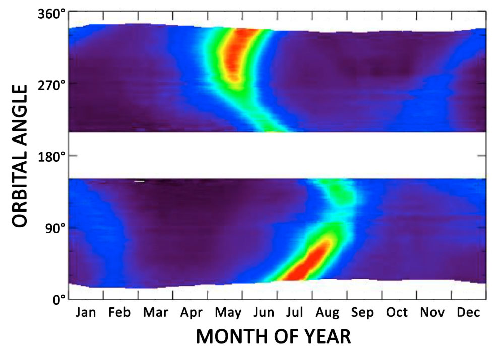
Examining V2 ascending versus descending data resulted in a more accurate "Geometric Optics" (GO) model for V3 (see Fig. 2), which takes into account orbit position (y-axis in the graph above - click to enlarge) versus month (x-axis). Red values are equivalent to corrections of 6 practical salinity units, 30 times the desired monthly accuracy of the Aquarius measurement.
The V3 data processing included a relatively minor adjustment of the antenna pattern. It improved data collected during "cold sky calibration" maneuvers, when the satellite observatory rotated 180 degrees from the normal Earth-viewing mode to measure space, which has a well-established and consistent temperature. Likewise, V3 better corrected for data collected from "hot" calibration scenes over land.
The Aquarius V3 data processing algorithm took better advantage of data collected by the onboard scatterometer, which was used to calculate ocean roughness concurrently with the radiometers' brightness temperature measurements. Like the radiometers, the scatterometer measured signals both in horizontal (H) and vertical (V) polarizations. Unlike the radiometers, which passively measured natural radiation from the ocean surface, the scatterometer actively emitted radar pulses. Ocean roughness is derived from the change in these signals after they "bounced" off the sea surface.
Extensive data analysis has shown that models using H-polarization data from the scatterometer and radiometers provide optimal performance in terms of correcting for surface roughness effects. For example, these models performed well on data collected from storms with very high winds and rain (e.g., Hurricane Katia in 2011). Thus the V3 data release algorithm featured a new roughness correction model, which helped to significantly improve the accuracy of Aquarius' salinity measurements.
Validation against in-water salinity measurements from the ARGO drifter network and output from computer model runs revealed the need for additional minor adjustments to V3 salinity data, which are correlated with sea surface temperature. The likely cause is small uncertainties in the radiative transfer model used in the data processing algorithm, which relates electromagnetic radiation to ocean surface properties. Thus in addition to a "standard" salinity product, V3 provided an "adjusted" salinity that has been fine tuned to sea surface temperature measurements obtained from other sources (e.g., buoys and satellite infrared sensors).
The Aquarius Cal/Val team also refined the V3 data processing algorithm to filter undetected radio frequency interference (RFI) and flagging or masking instances of degraded algorithm performance (e.g., presence of sea ice, very high wind speeds, etc.).
Thanks to V3, this team was well "prepped" for yet another set of challenges. Click here to learn about the updates in Version 4 (V4) of the Aquarius data processing.