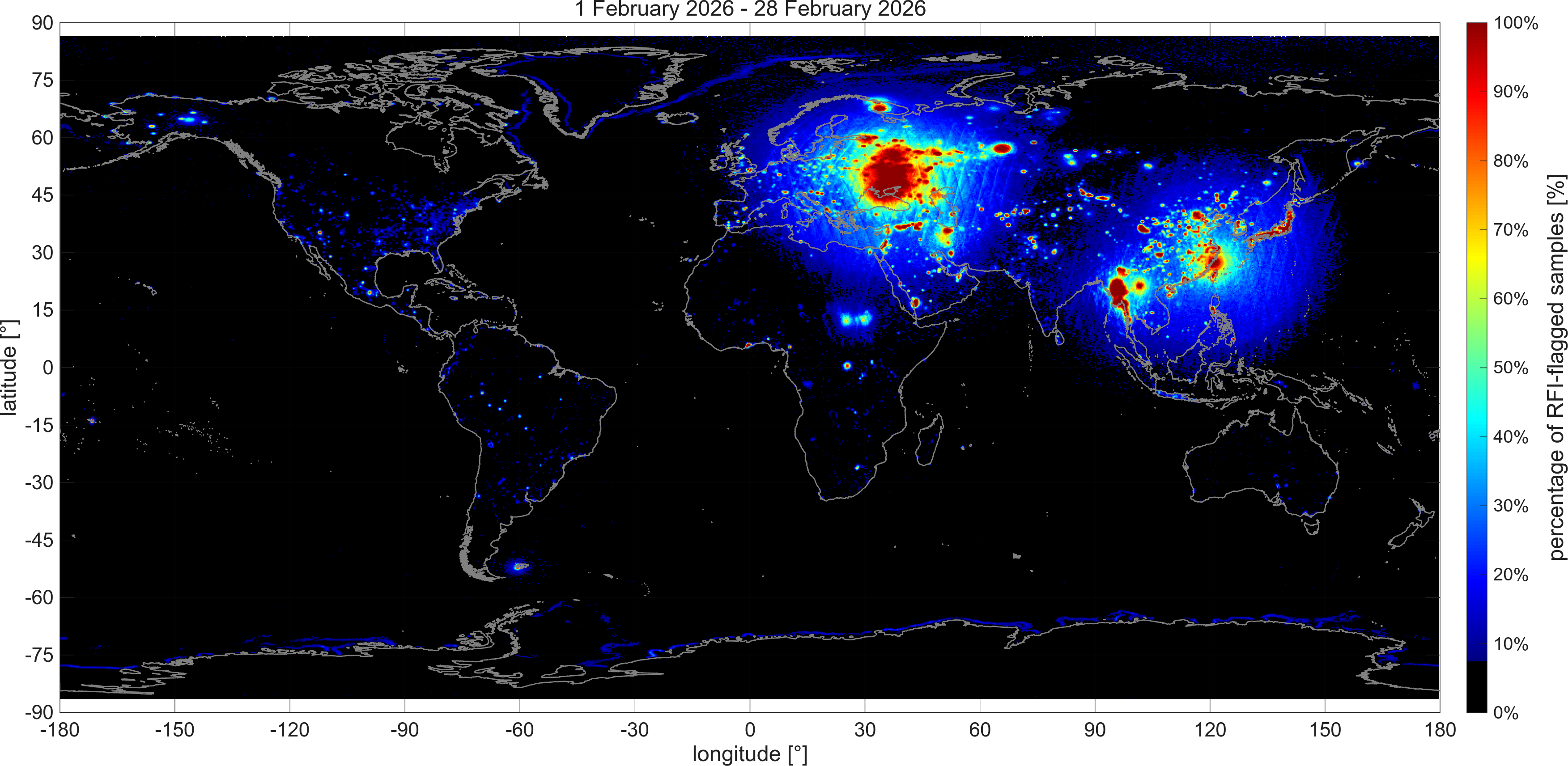
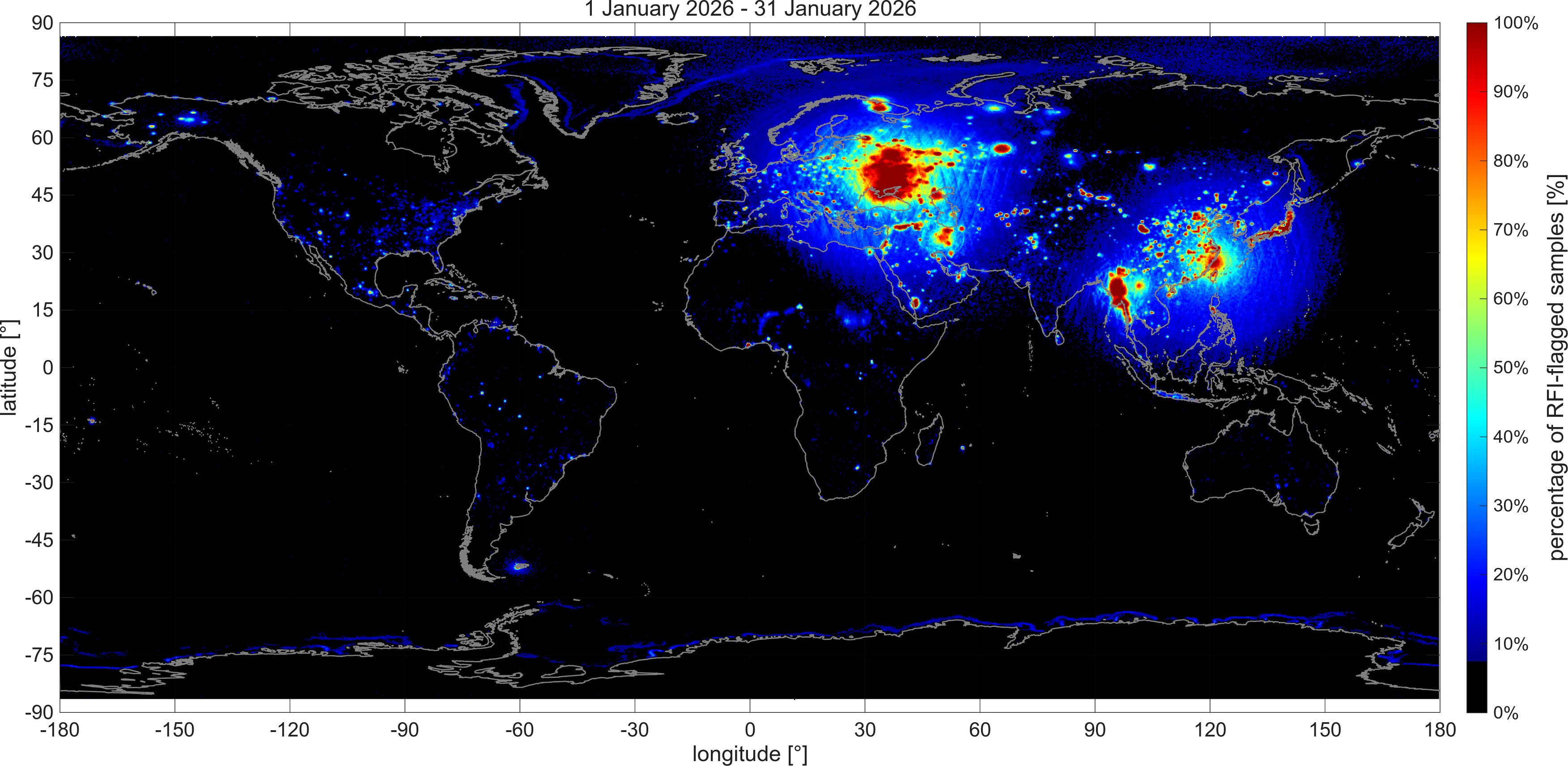
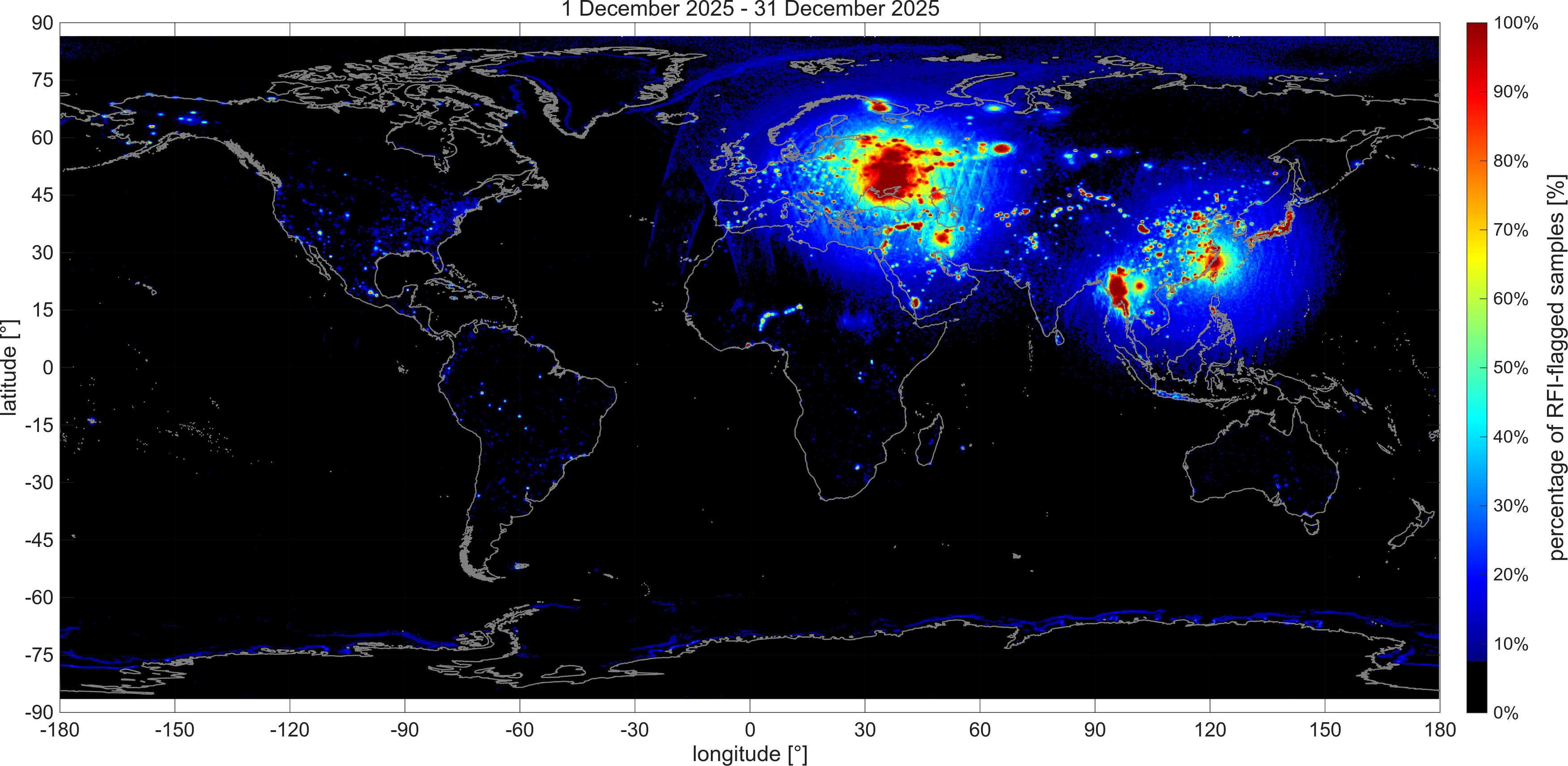
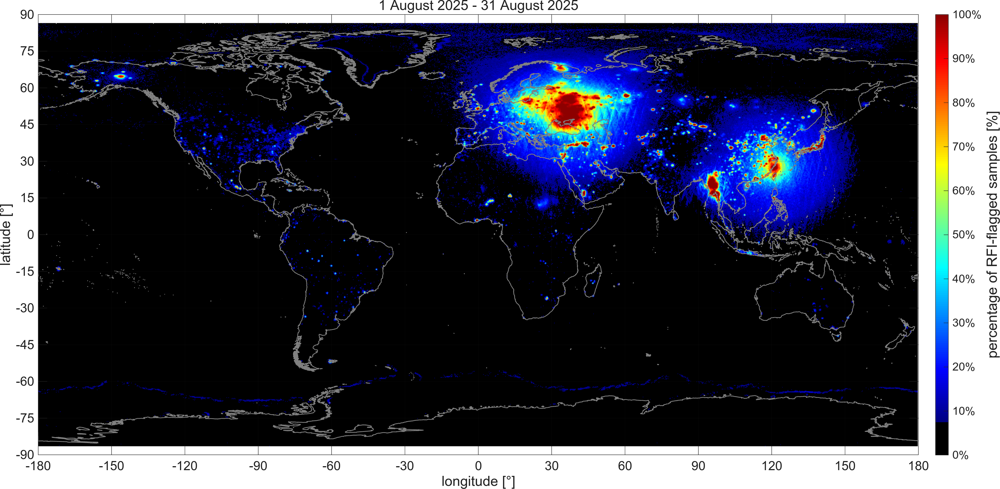
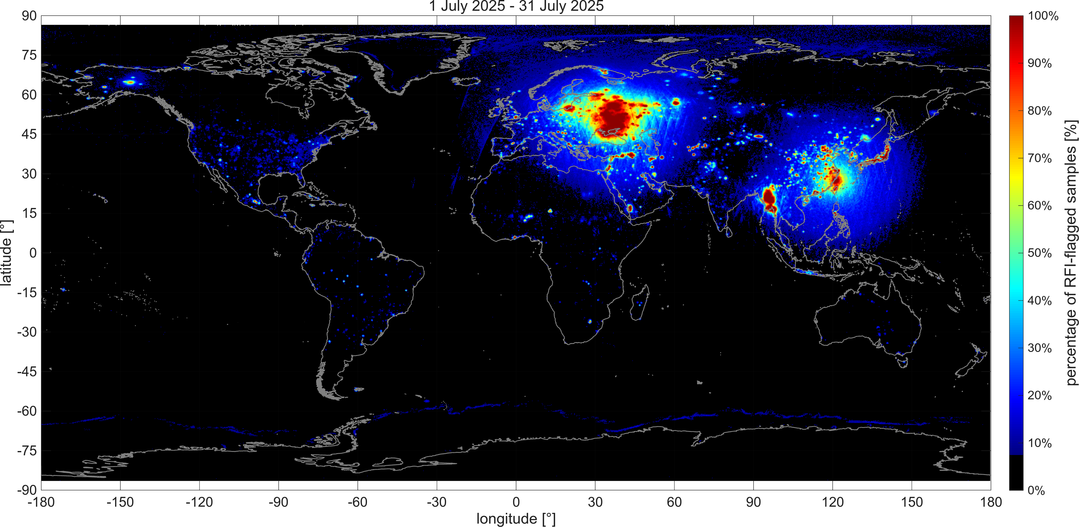
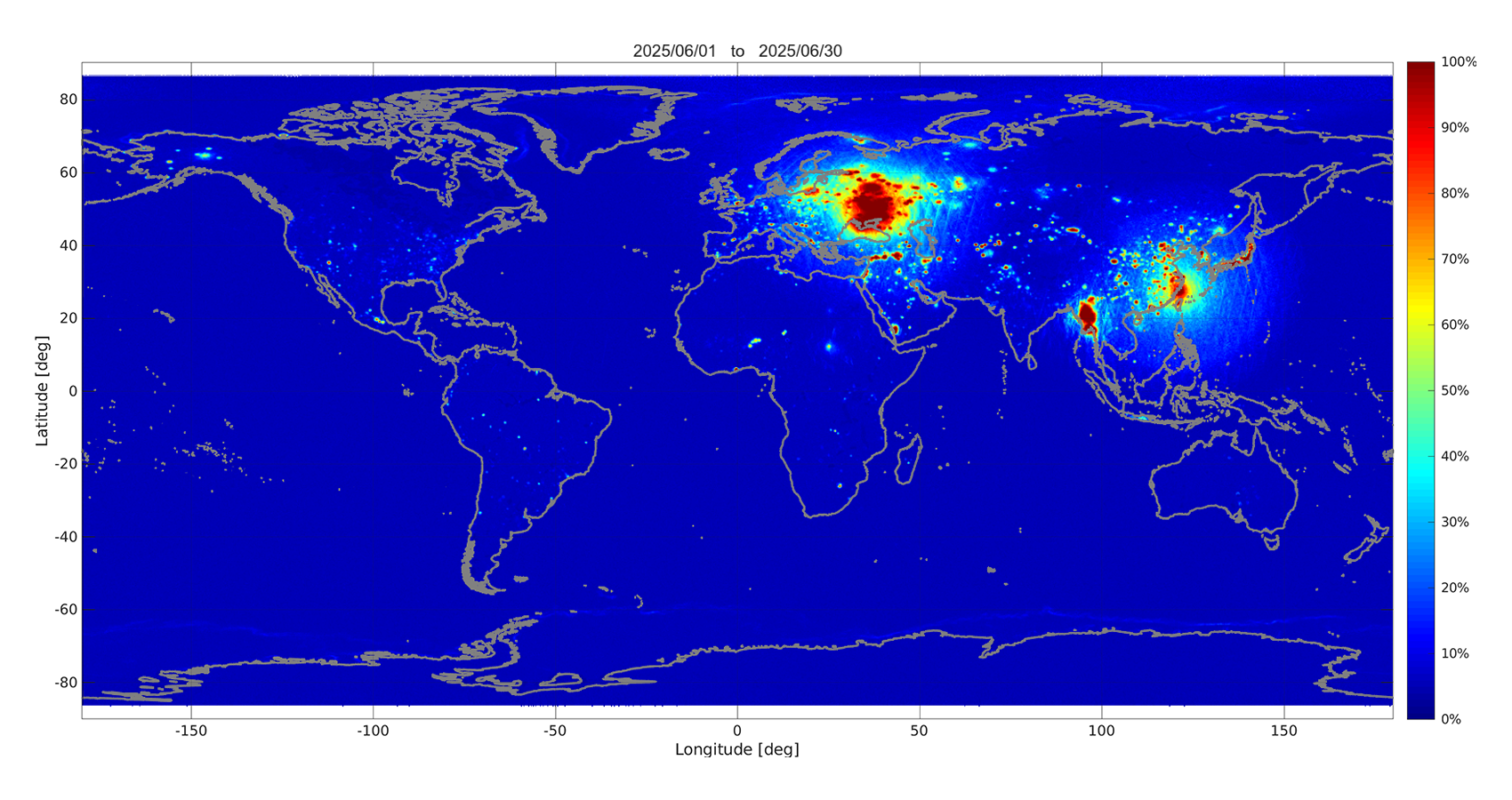
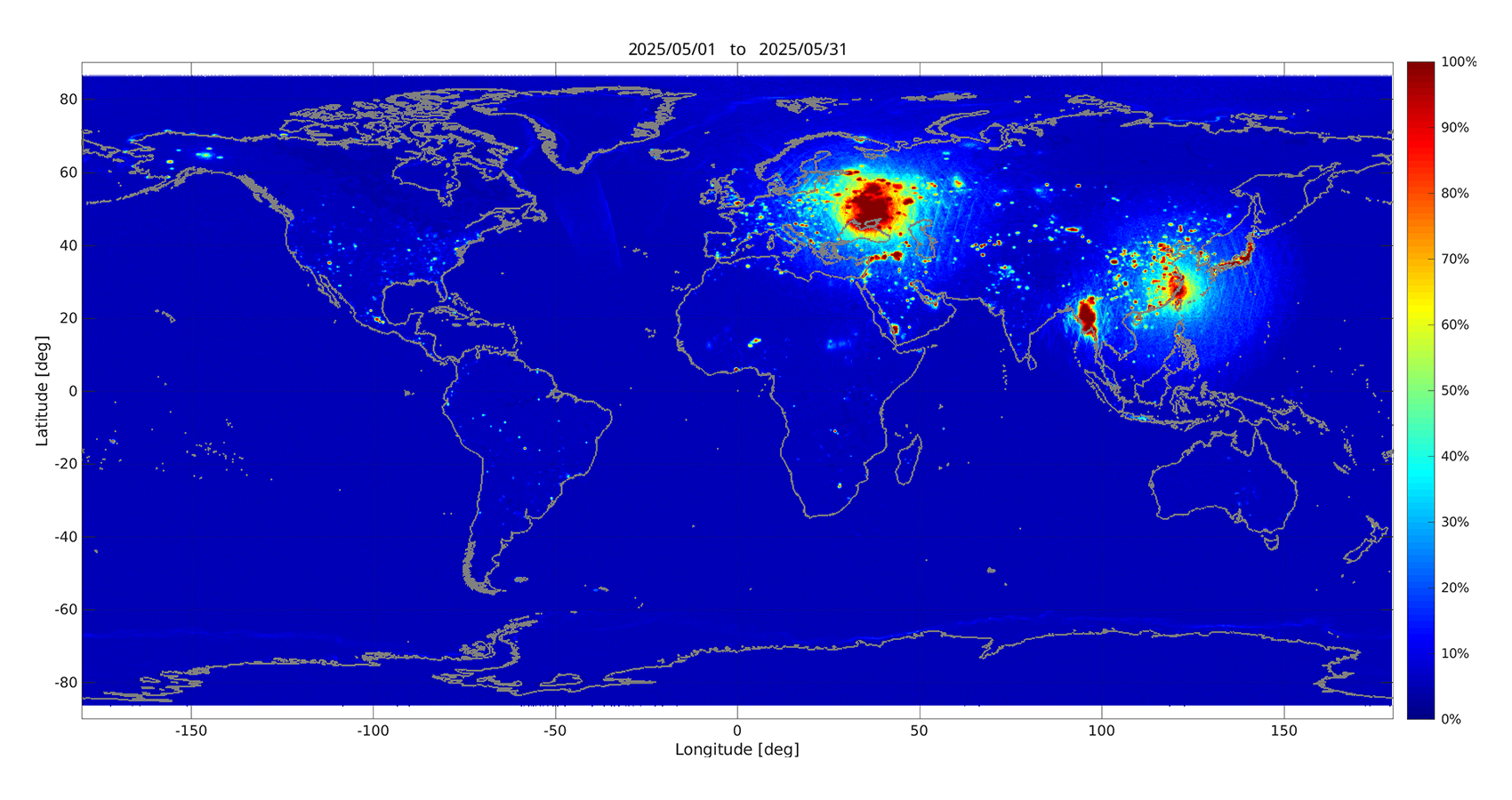
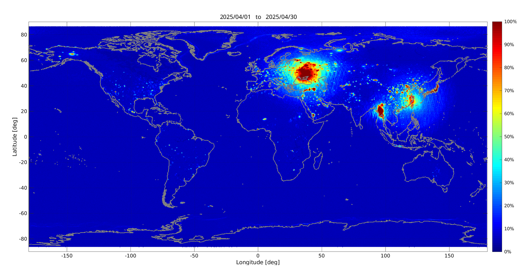
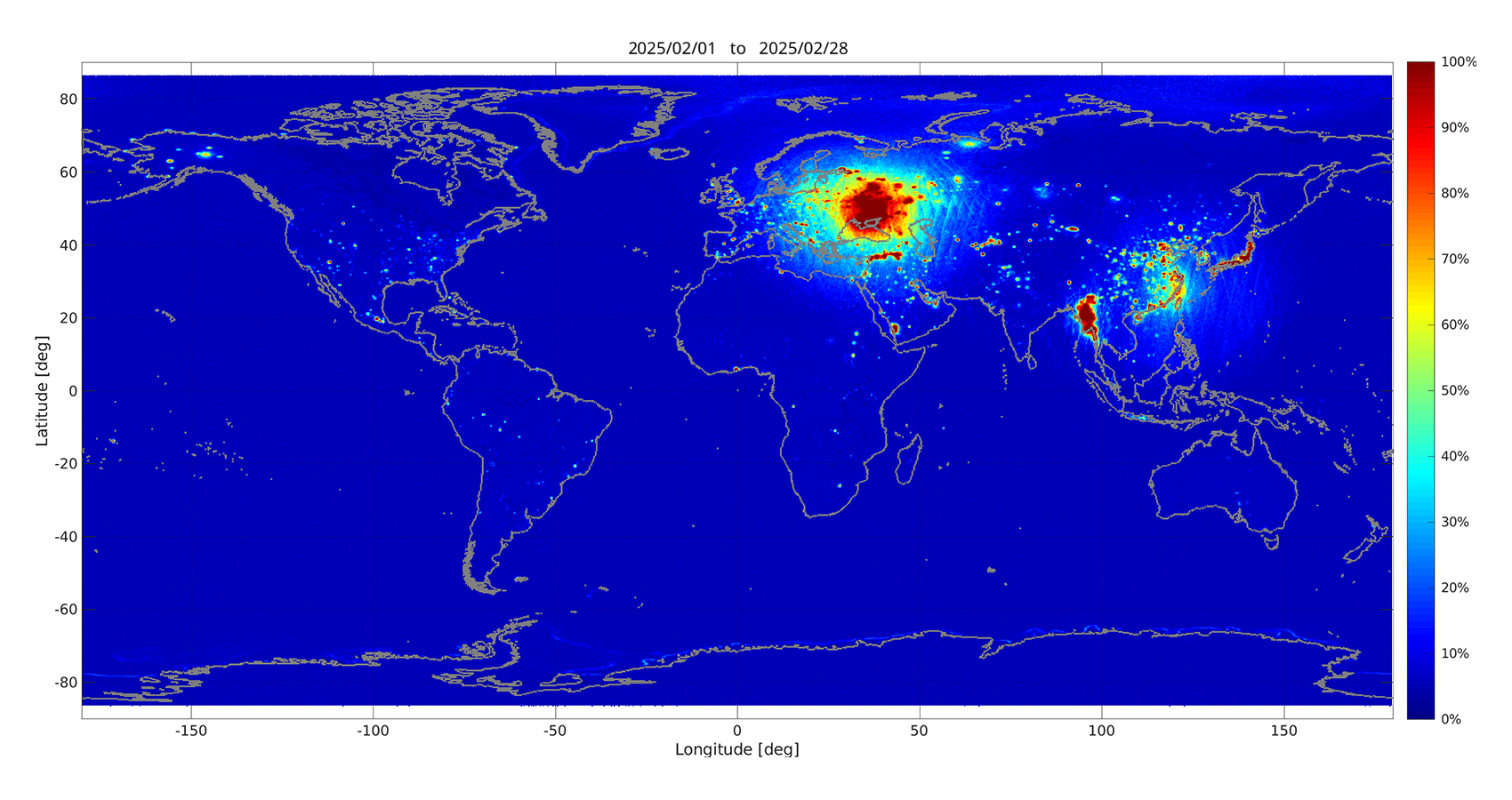
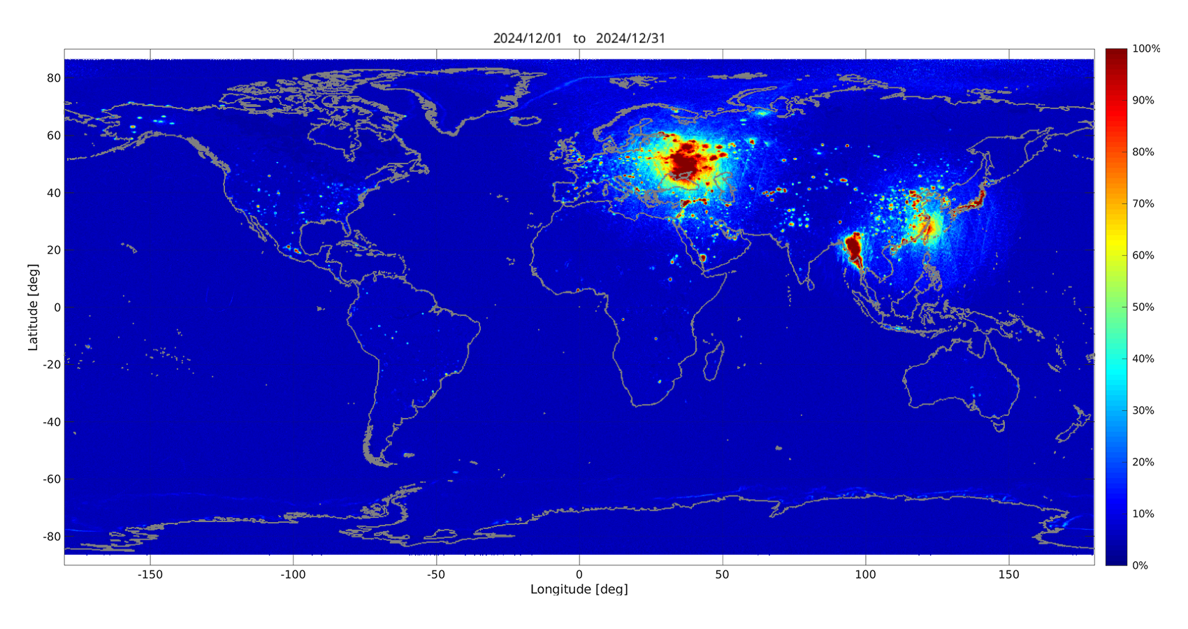
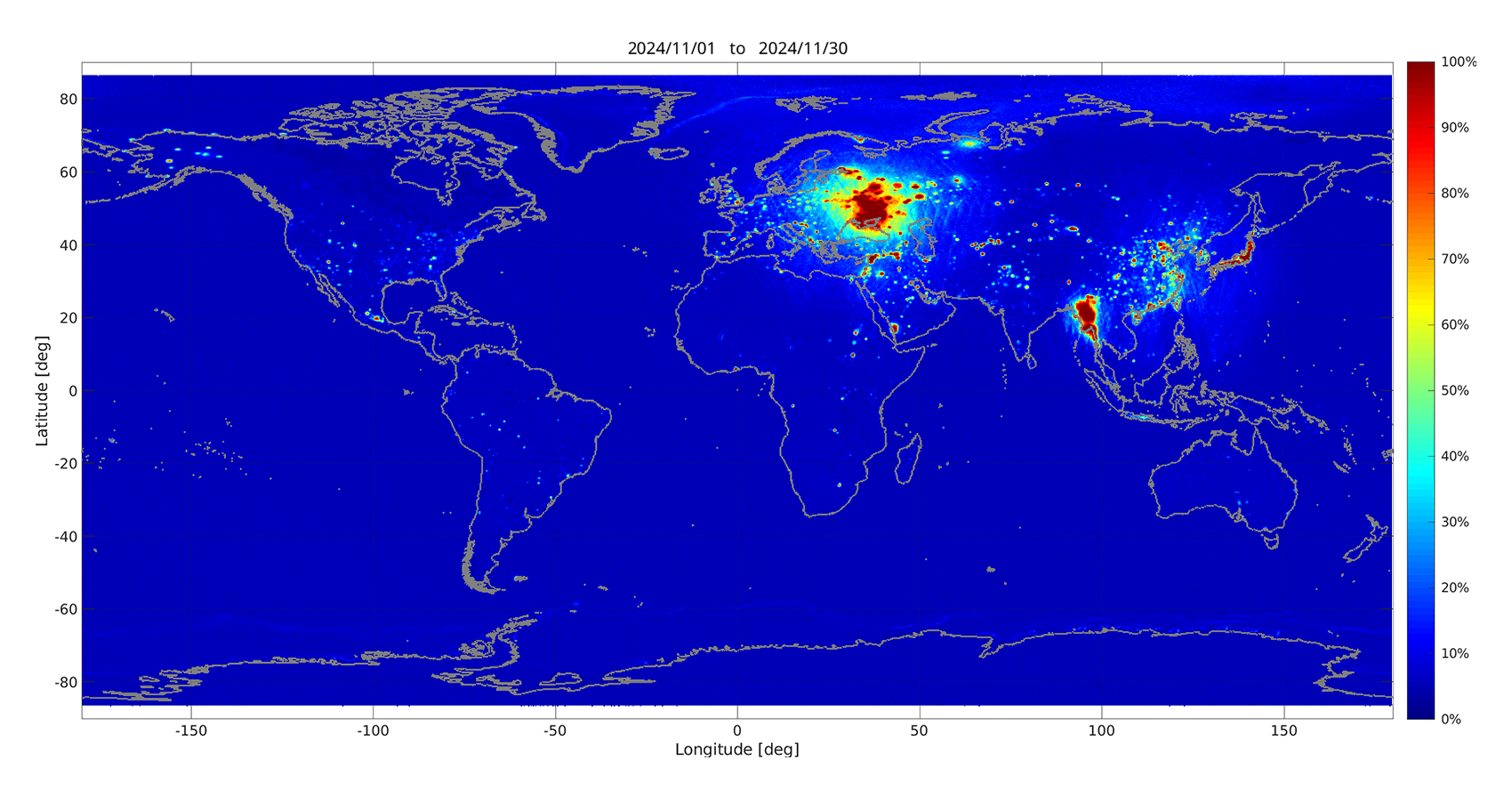
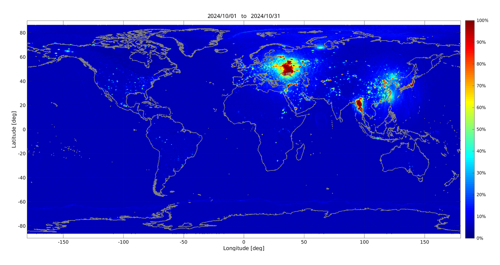
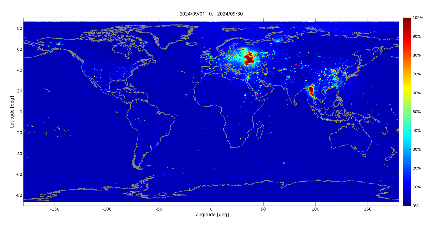
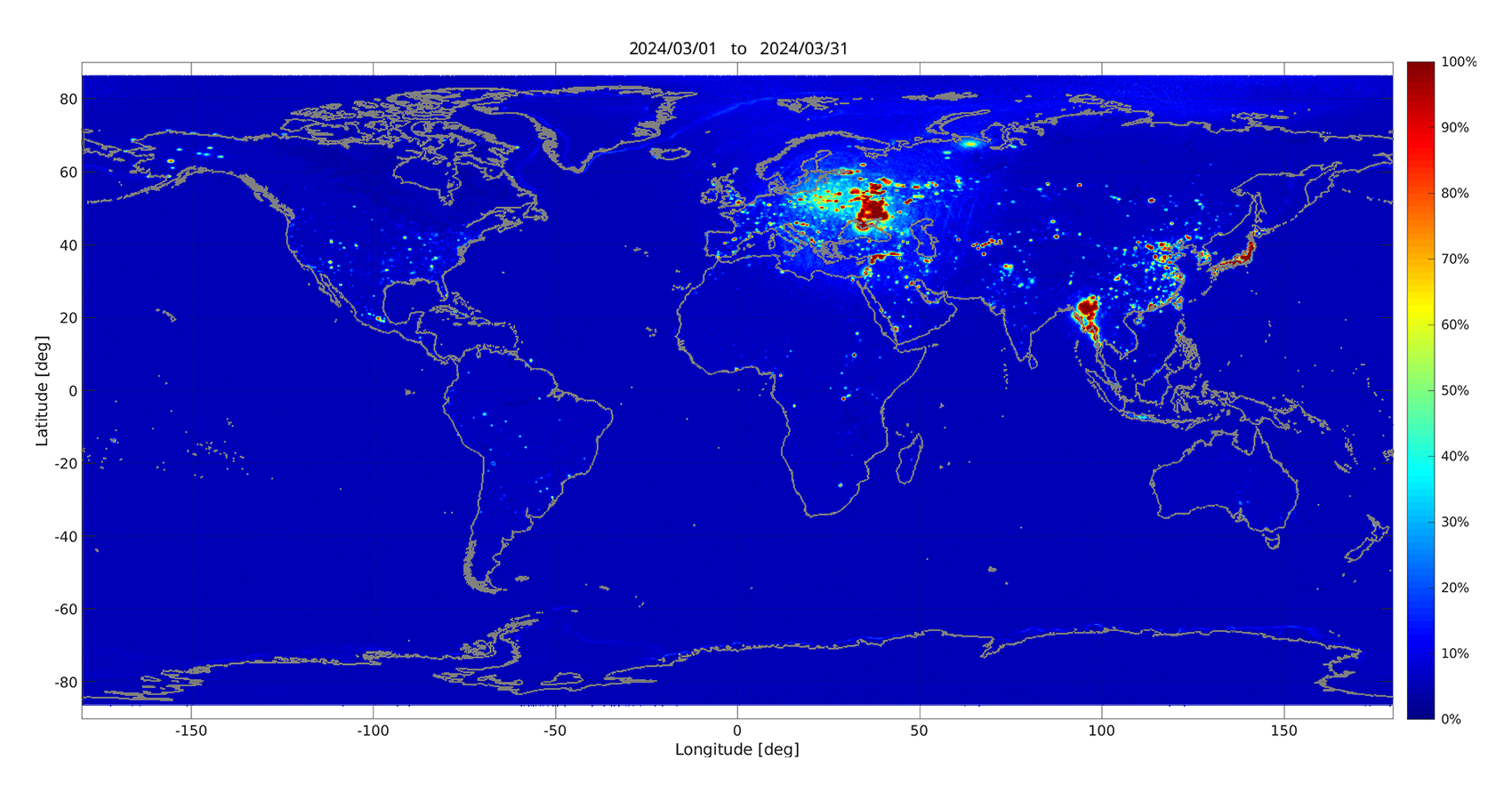
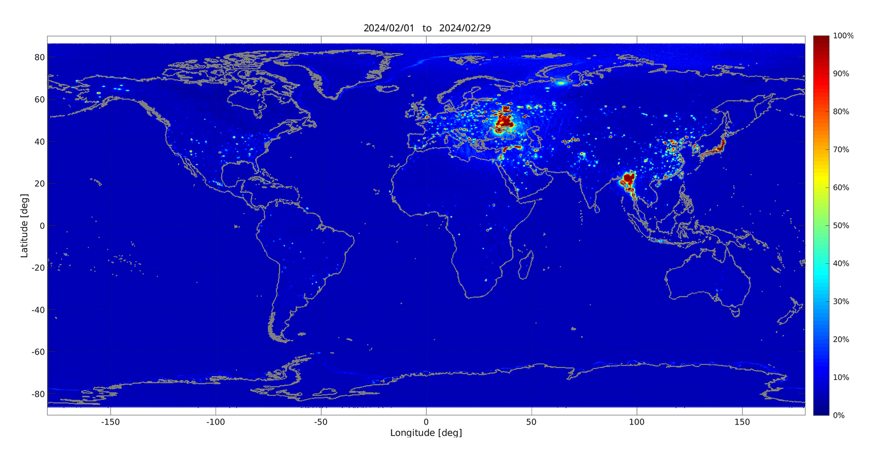
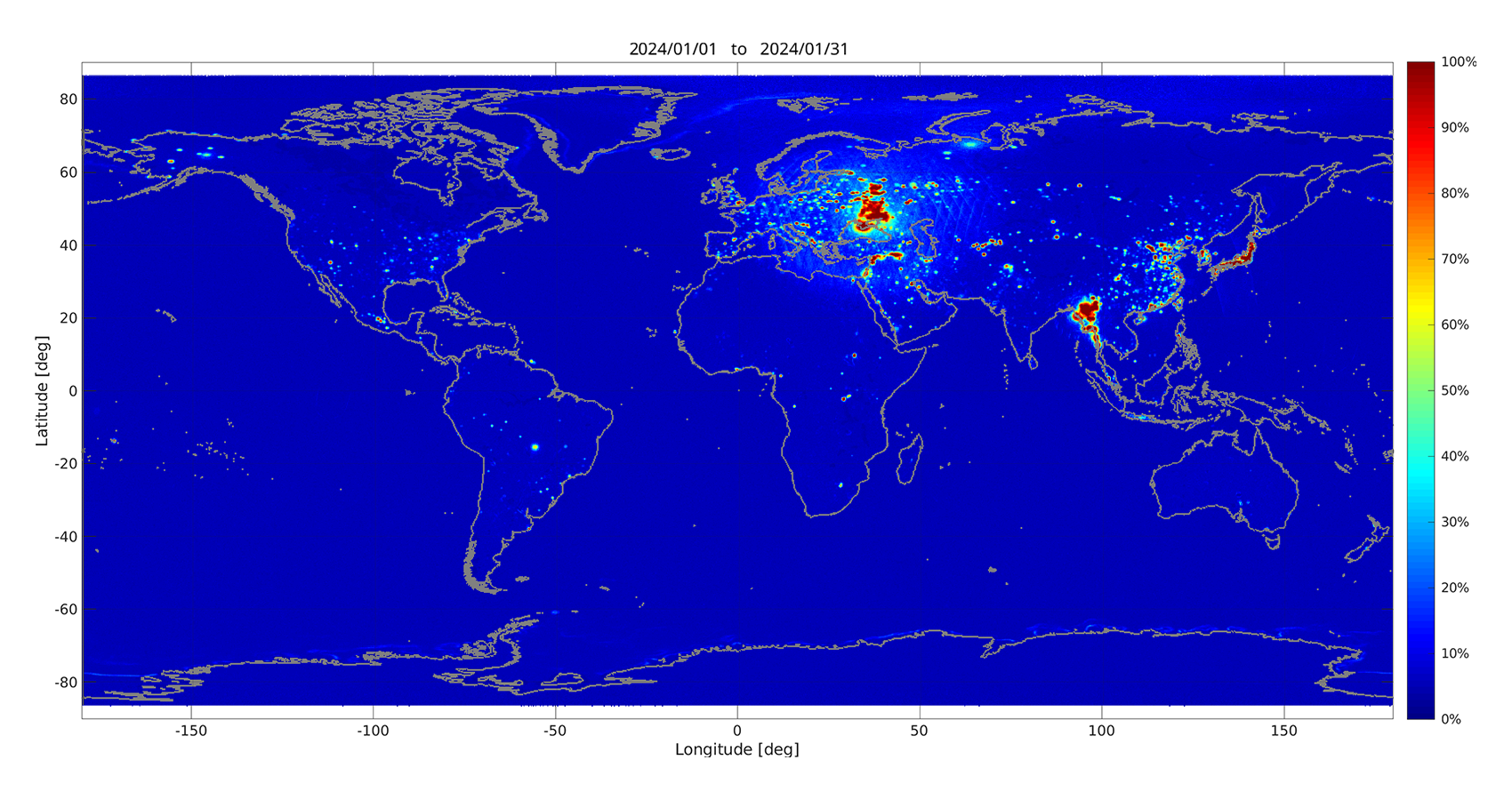
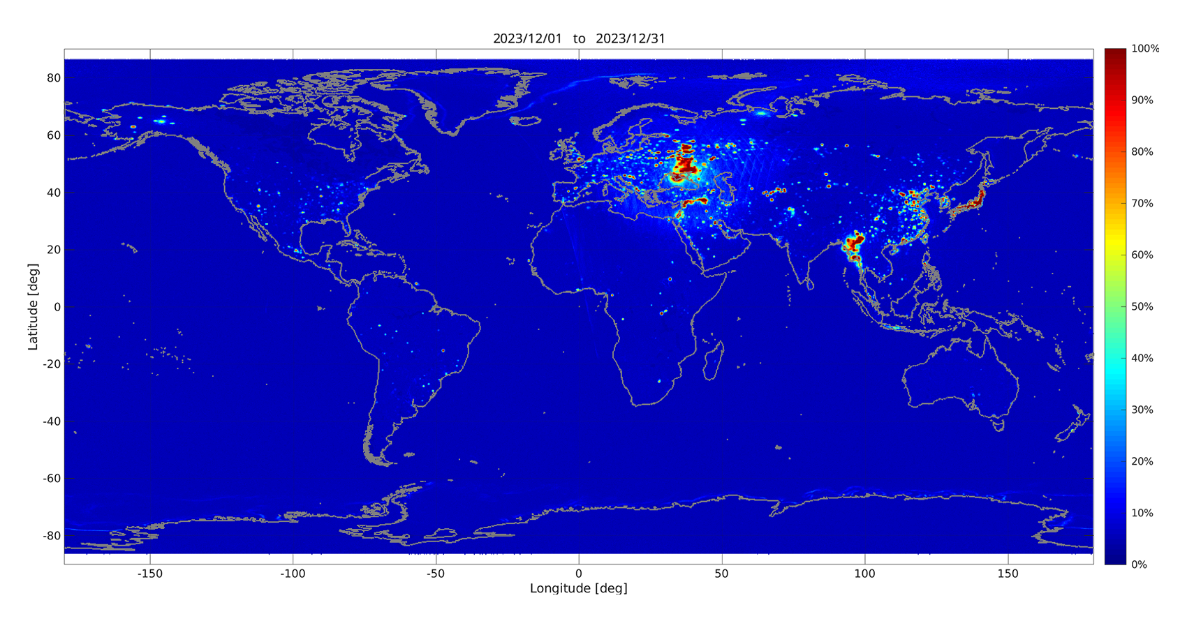
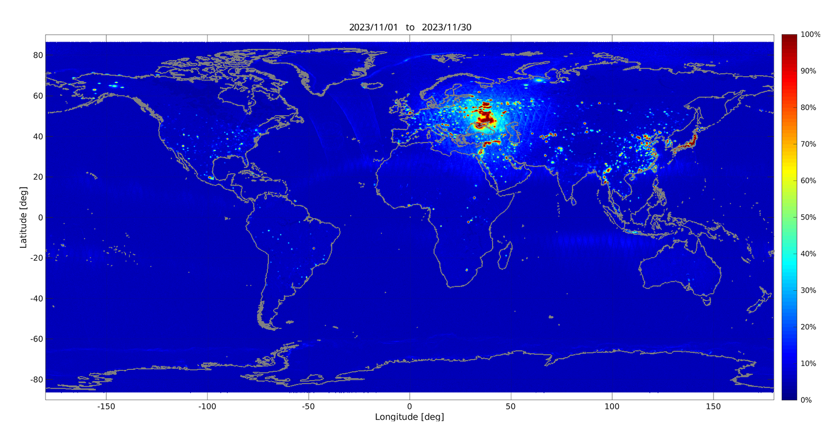
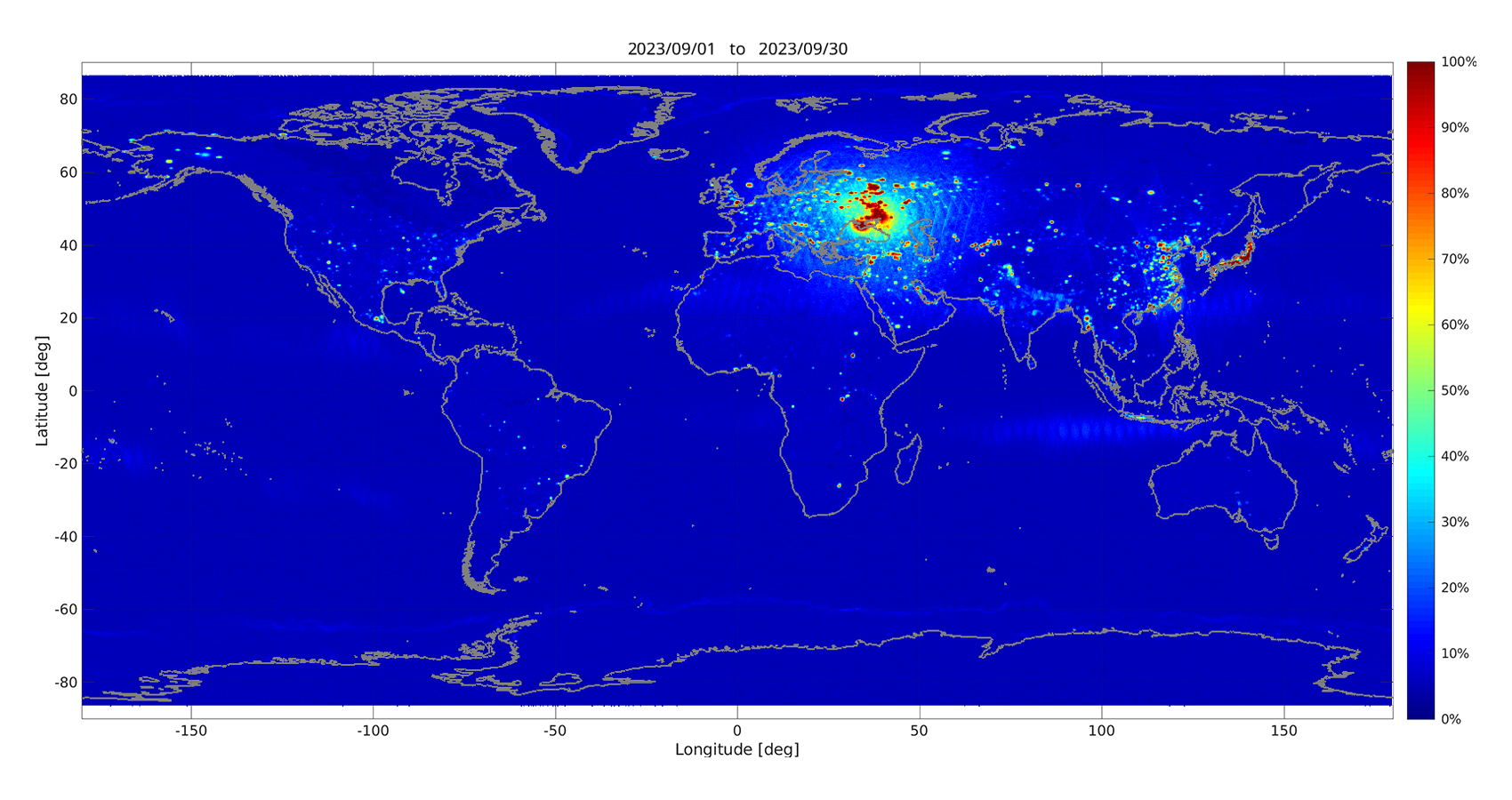
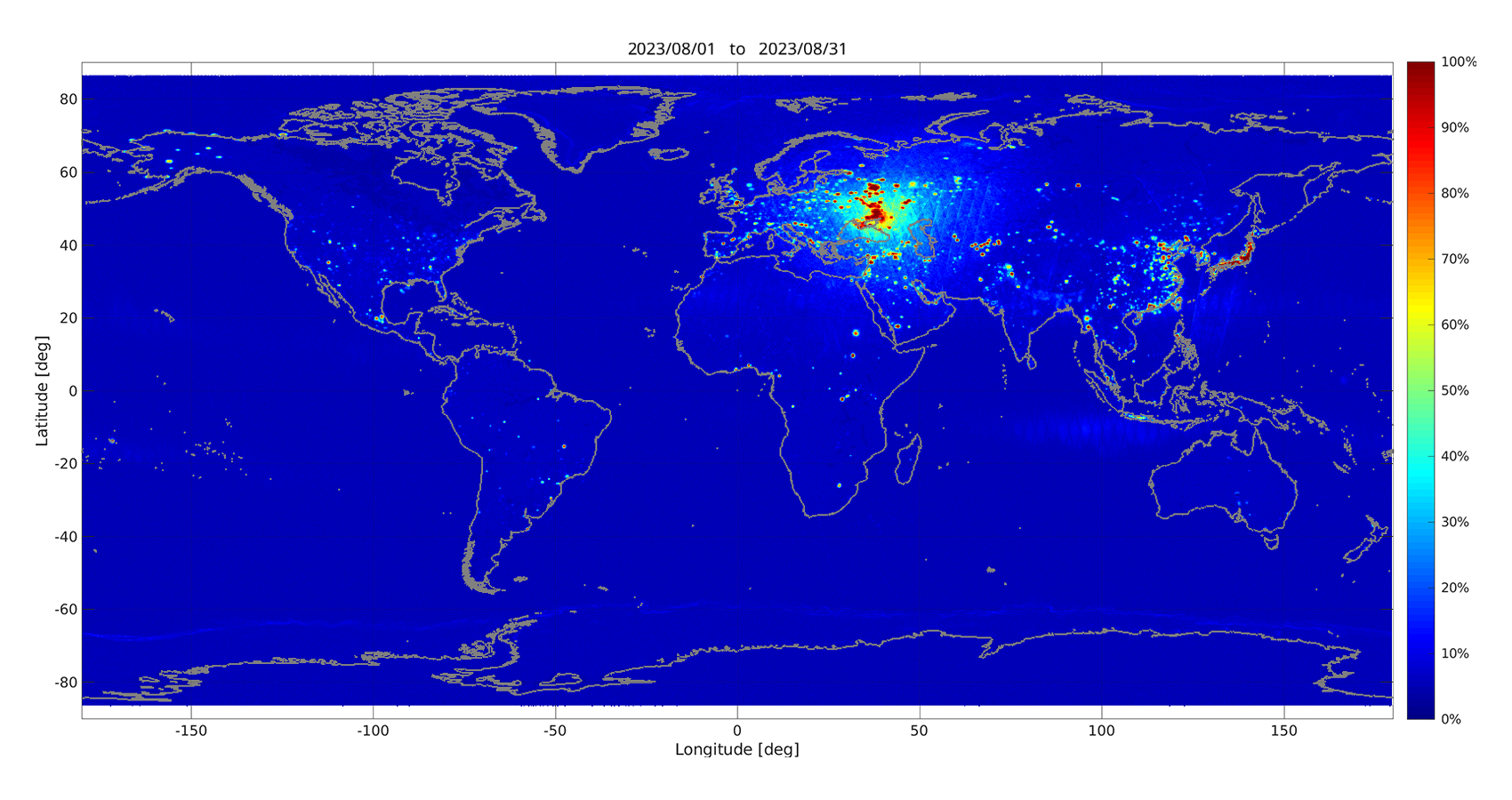
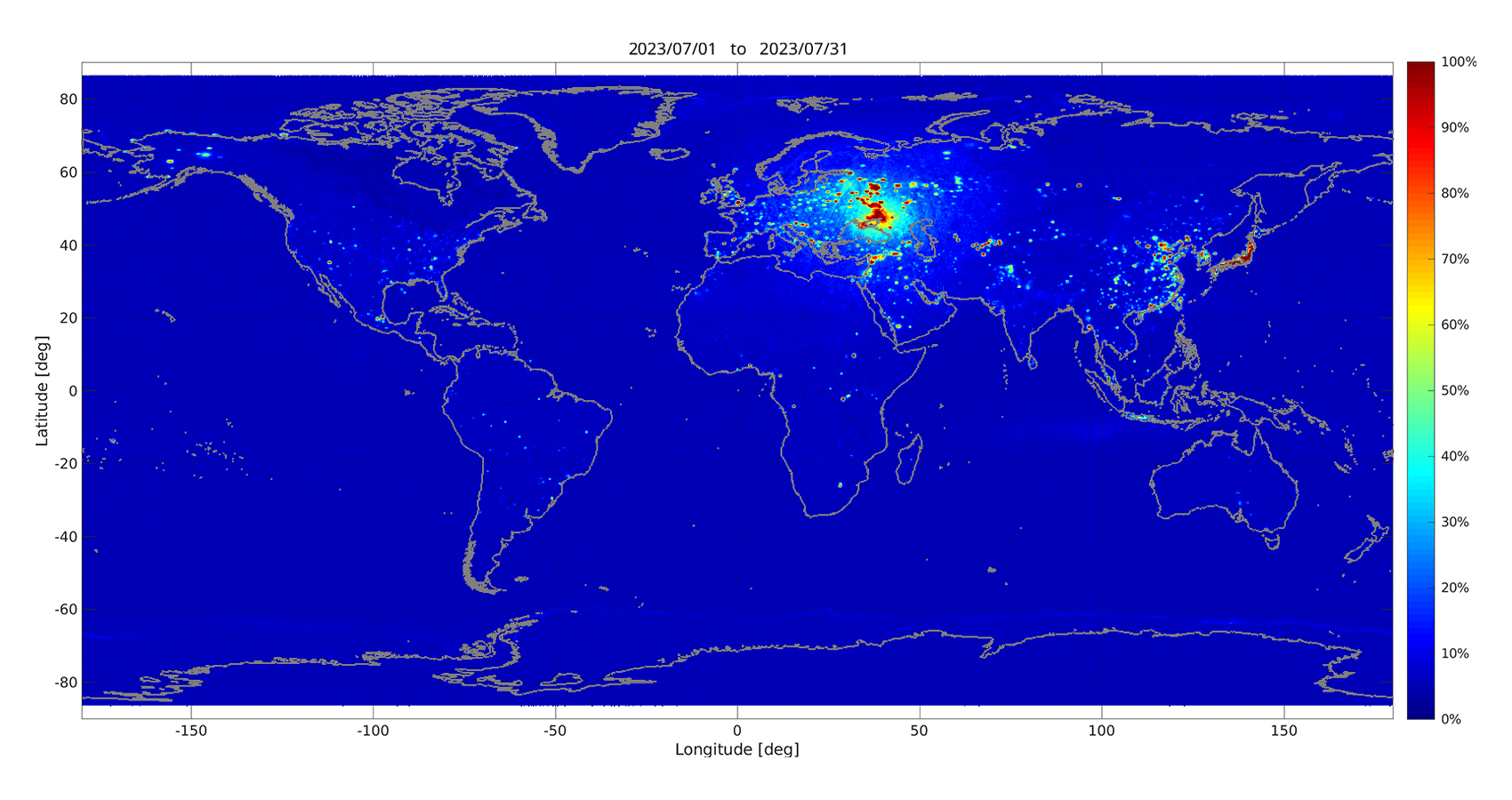
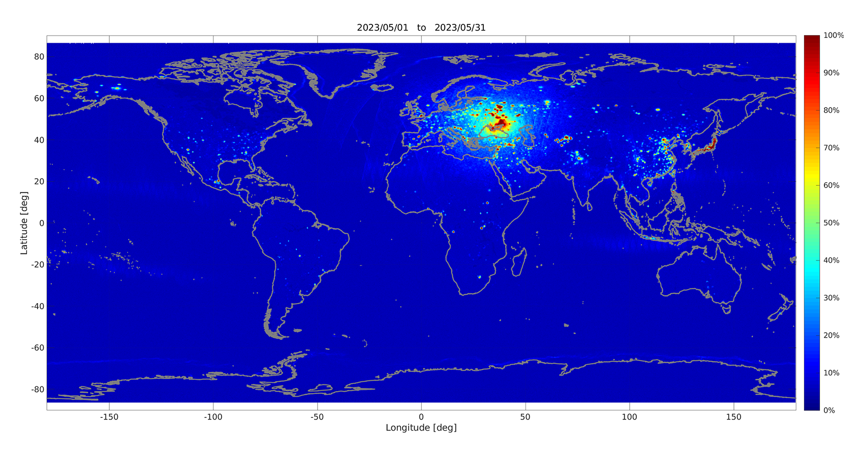
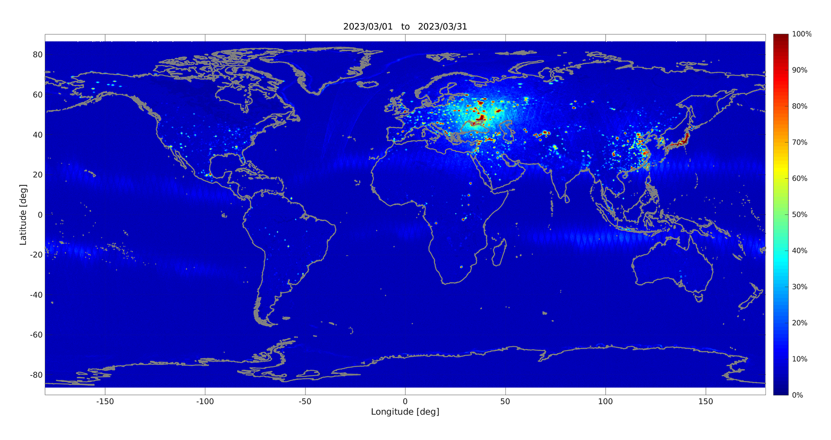
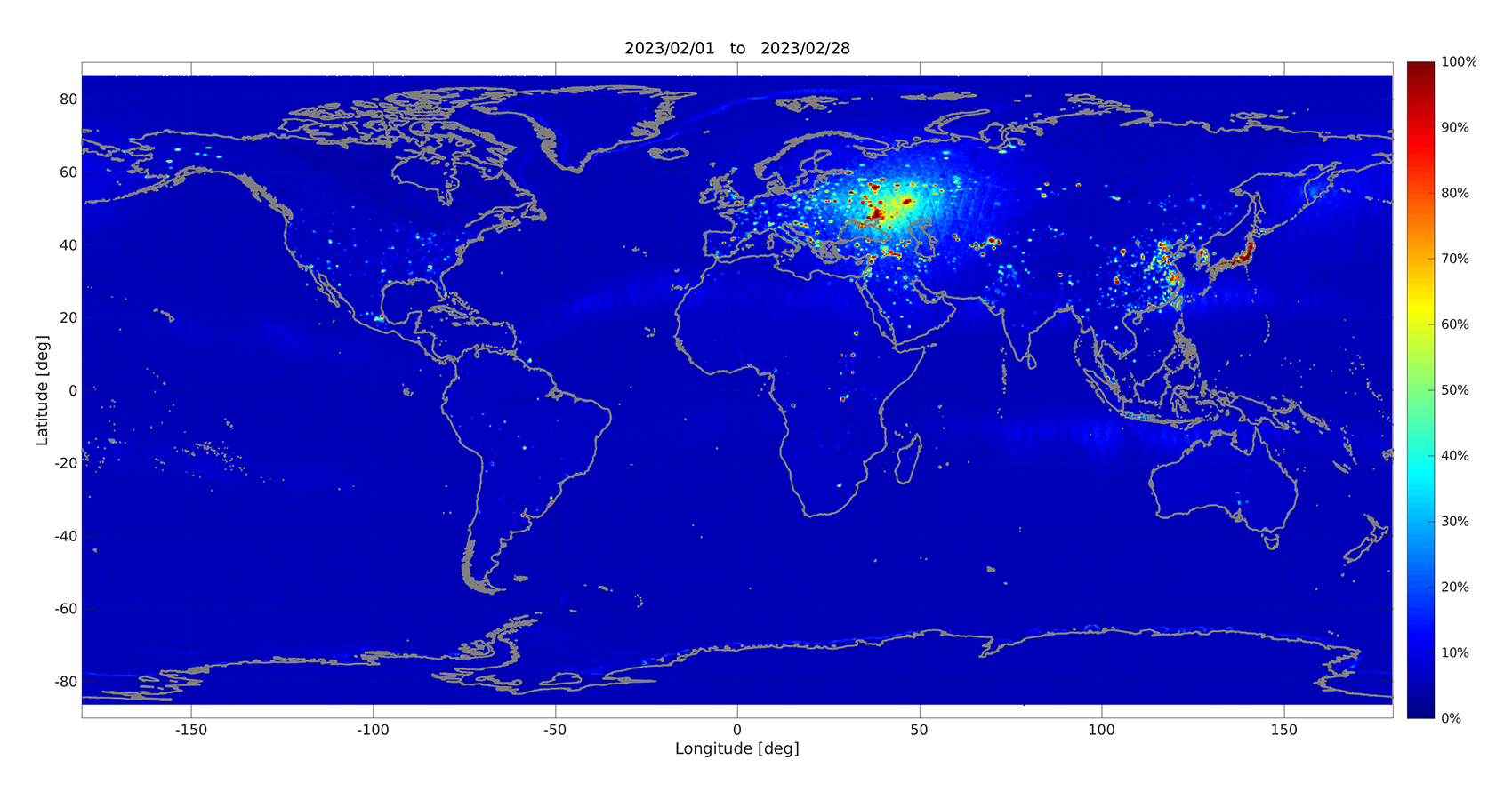
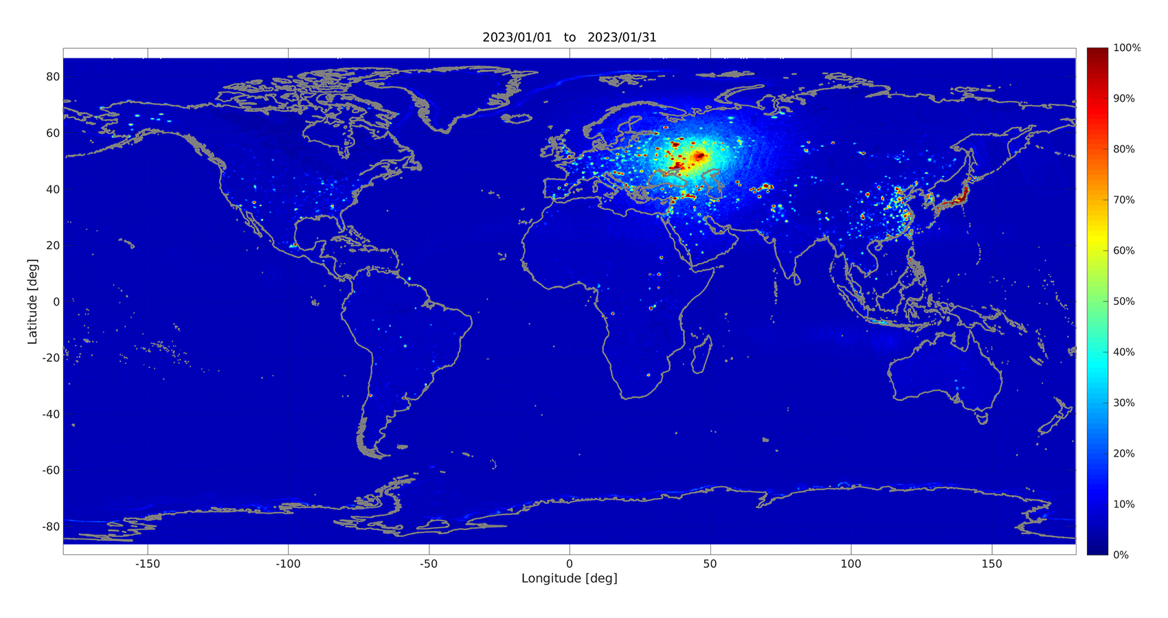
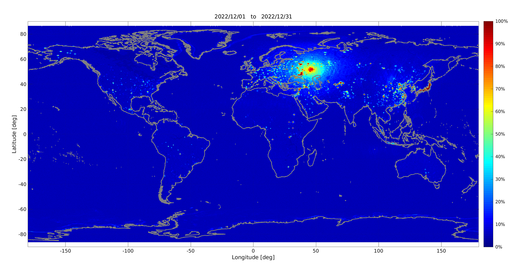
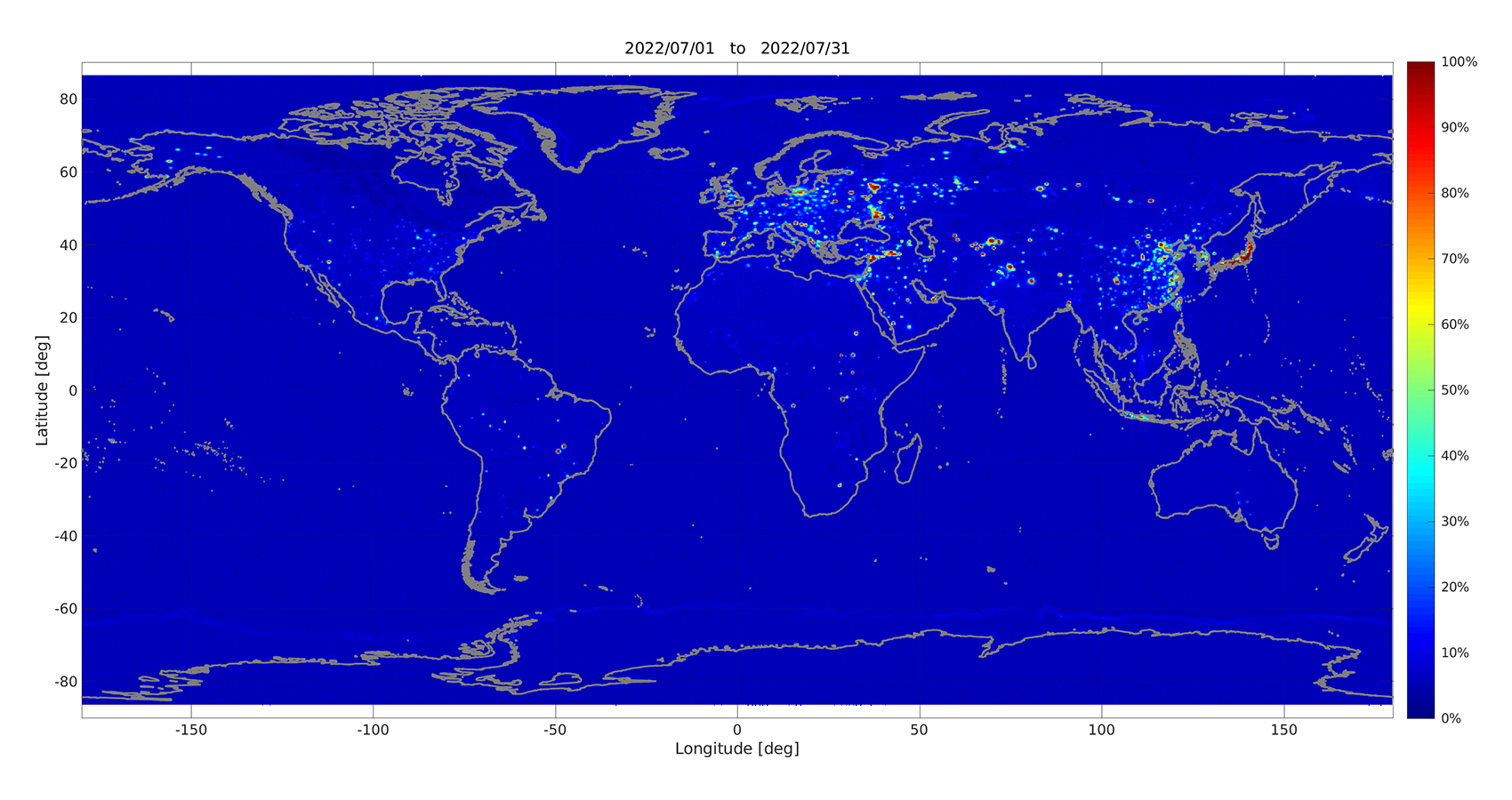
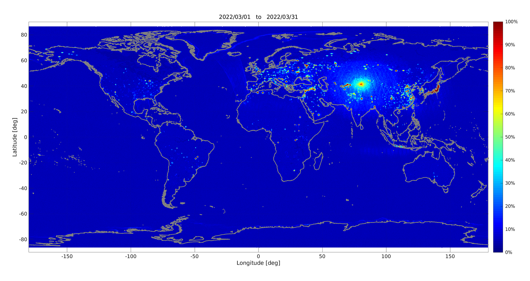
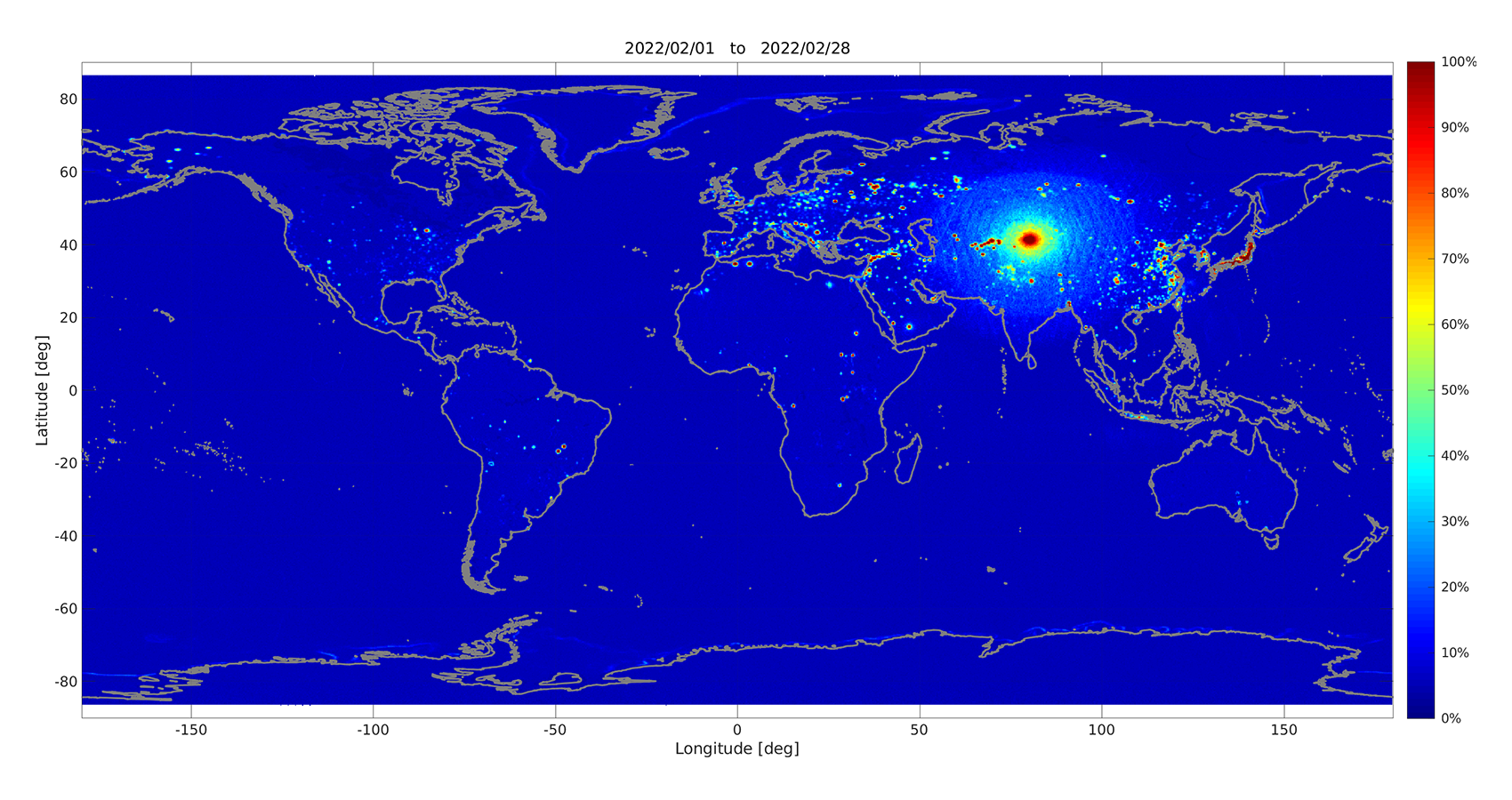
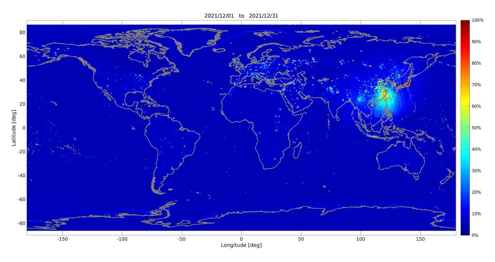
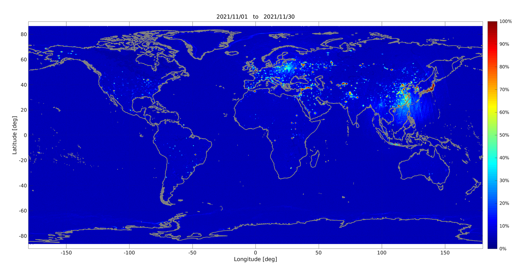
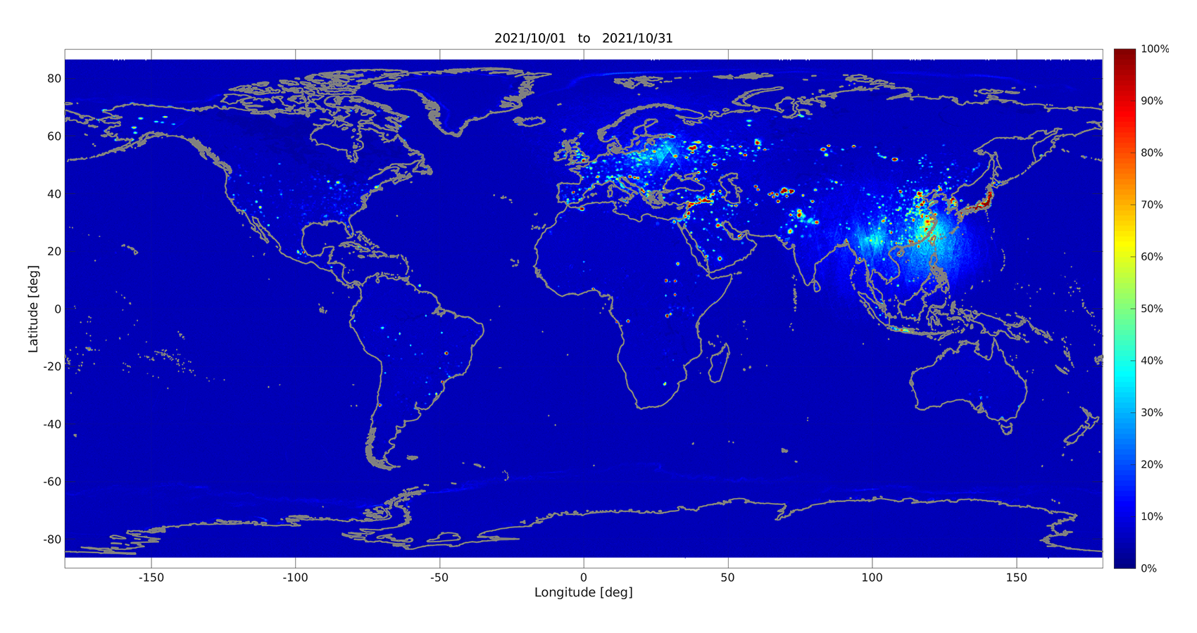
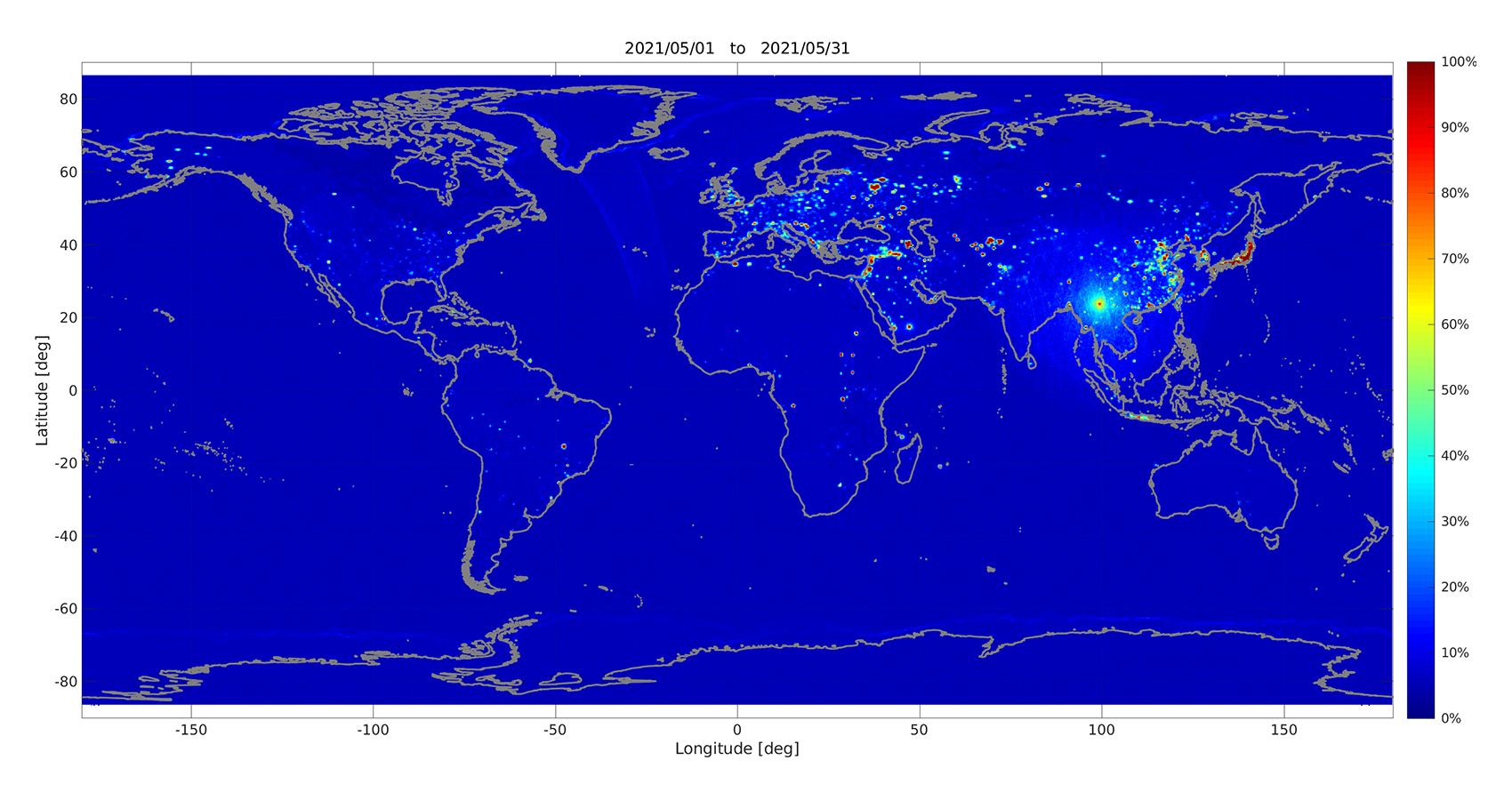
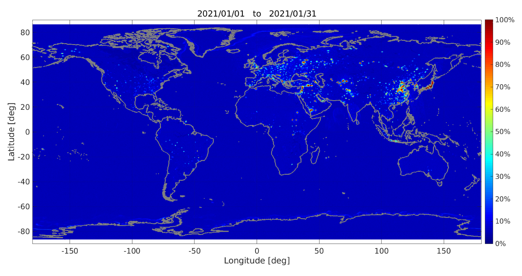
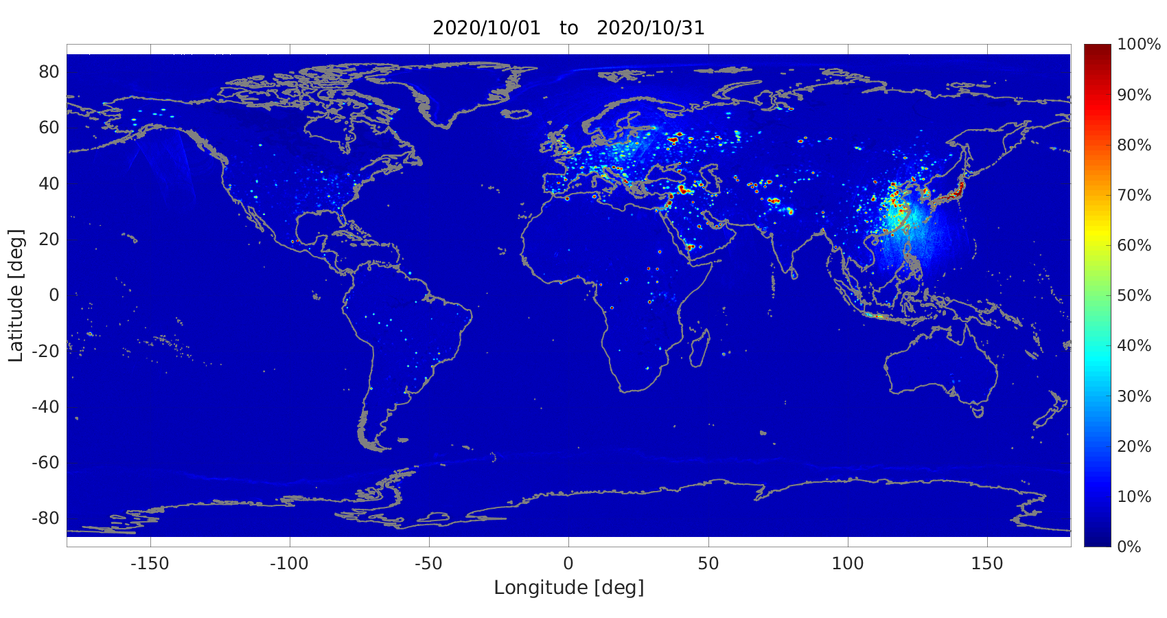
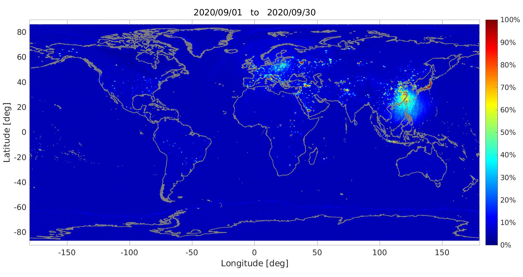
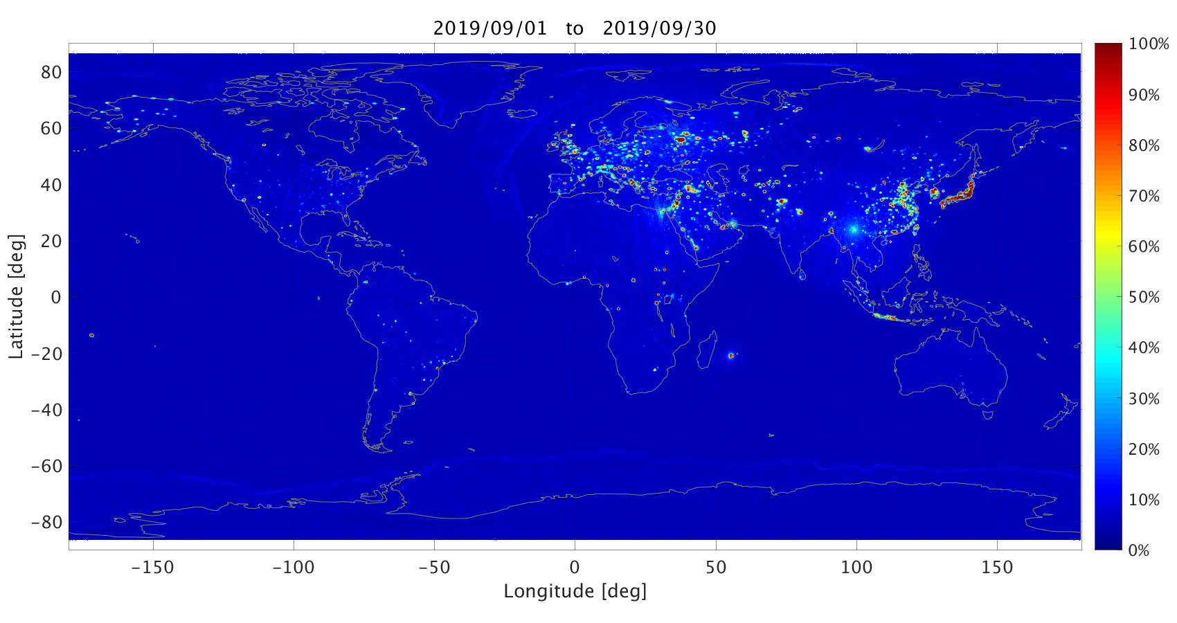
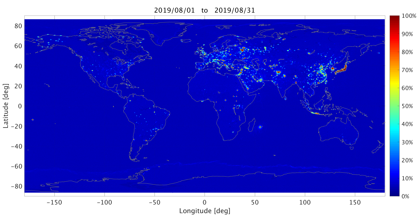
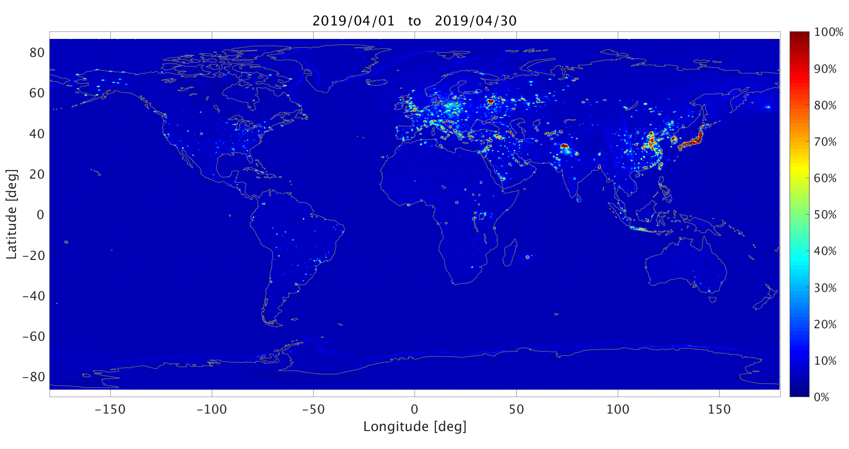
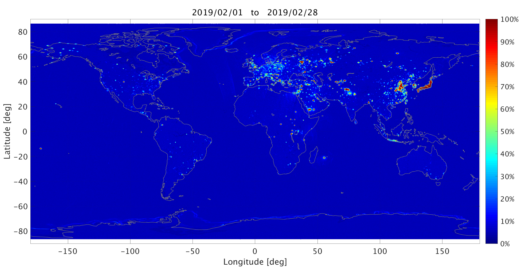
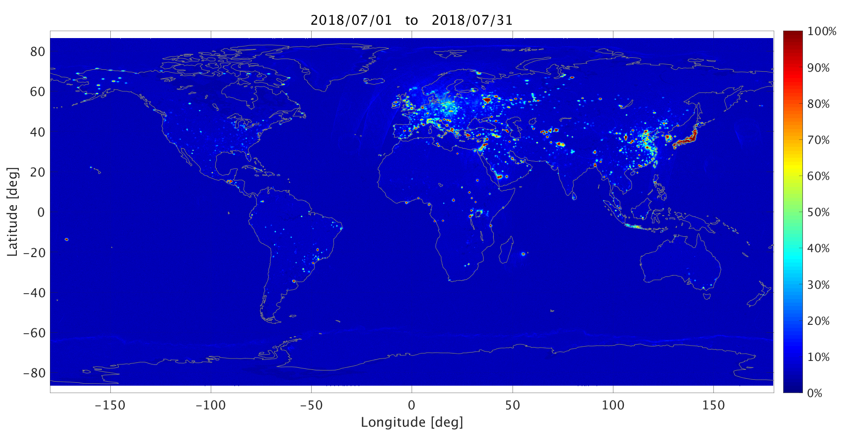
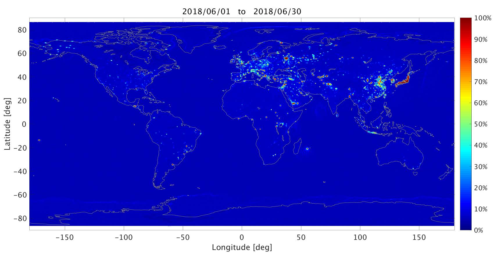
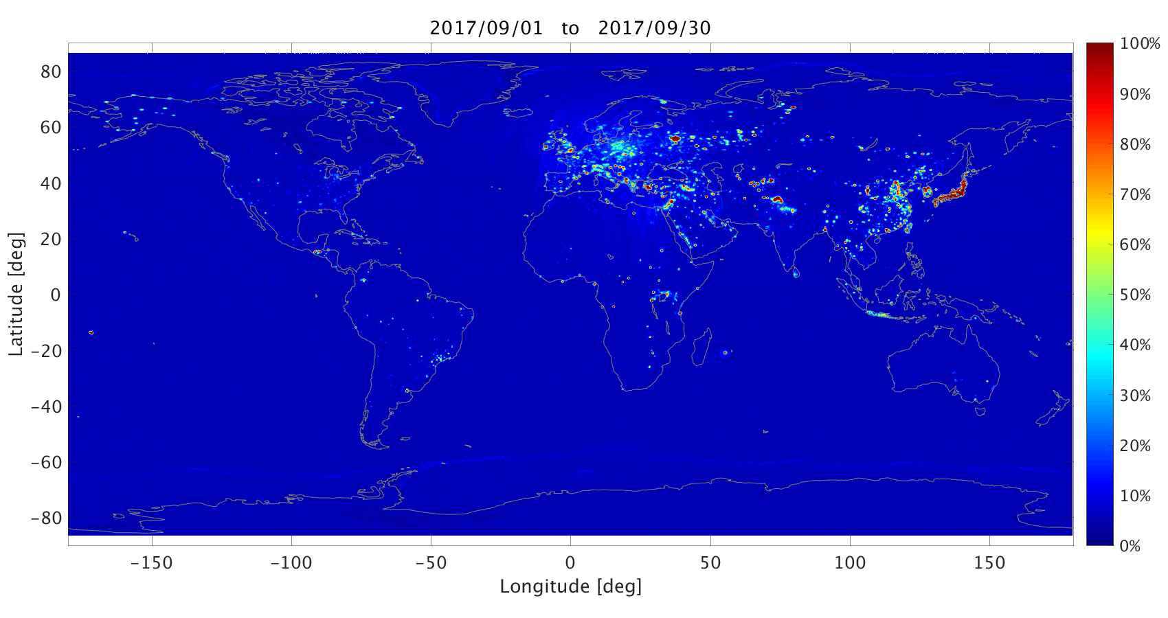
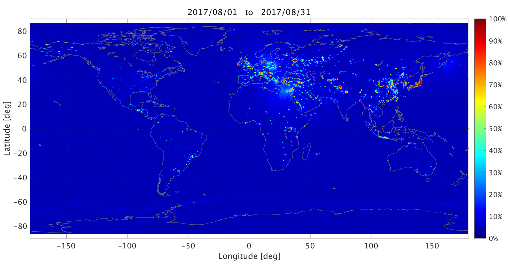
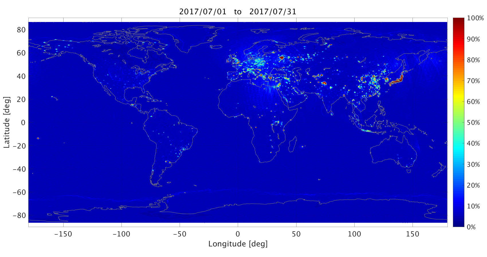
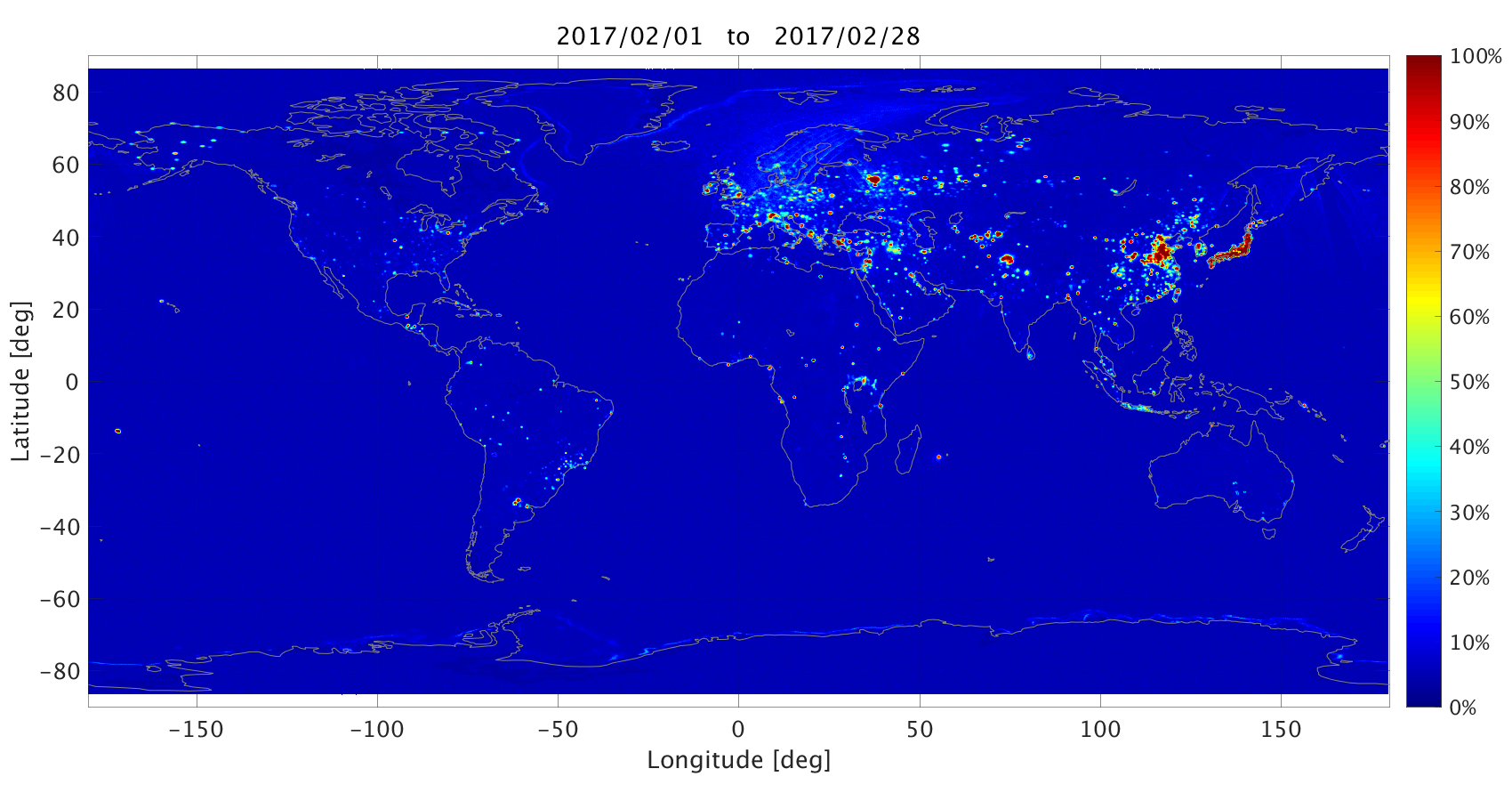
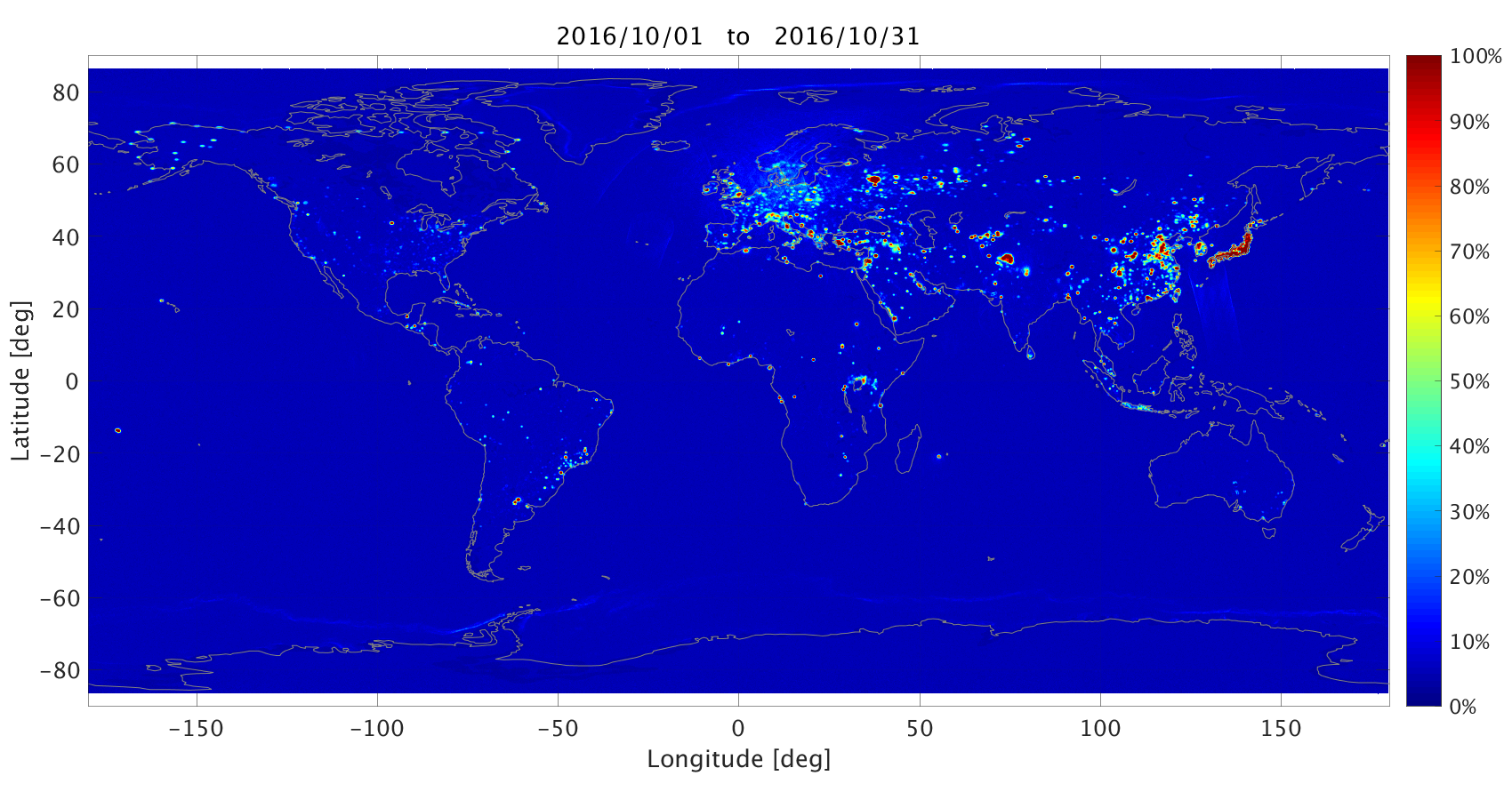
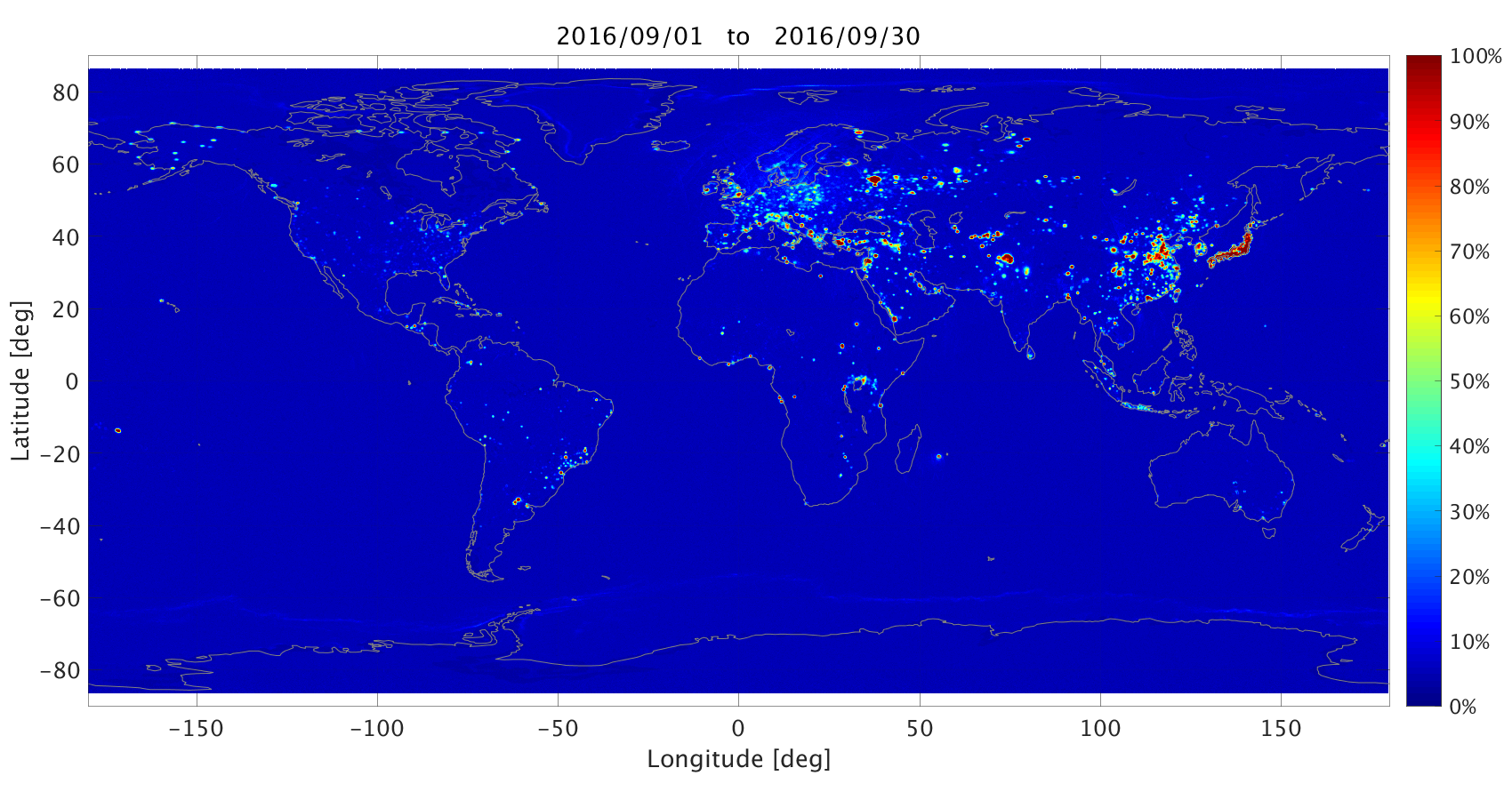
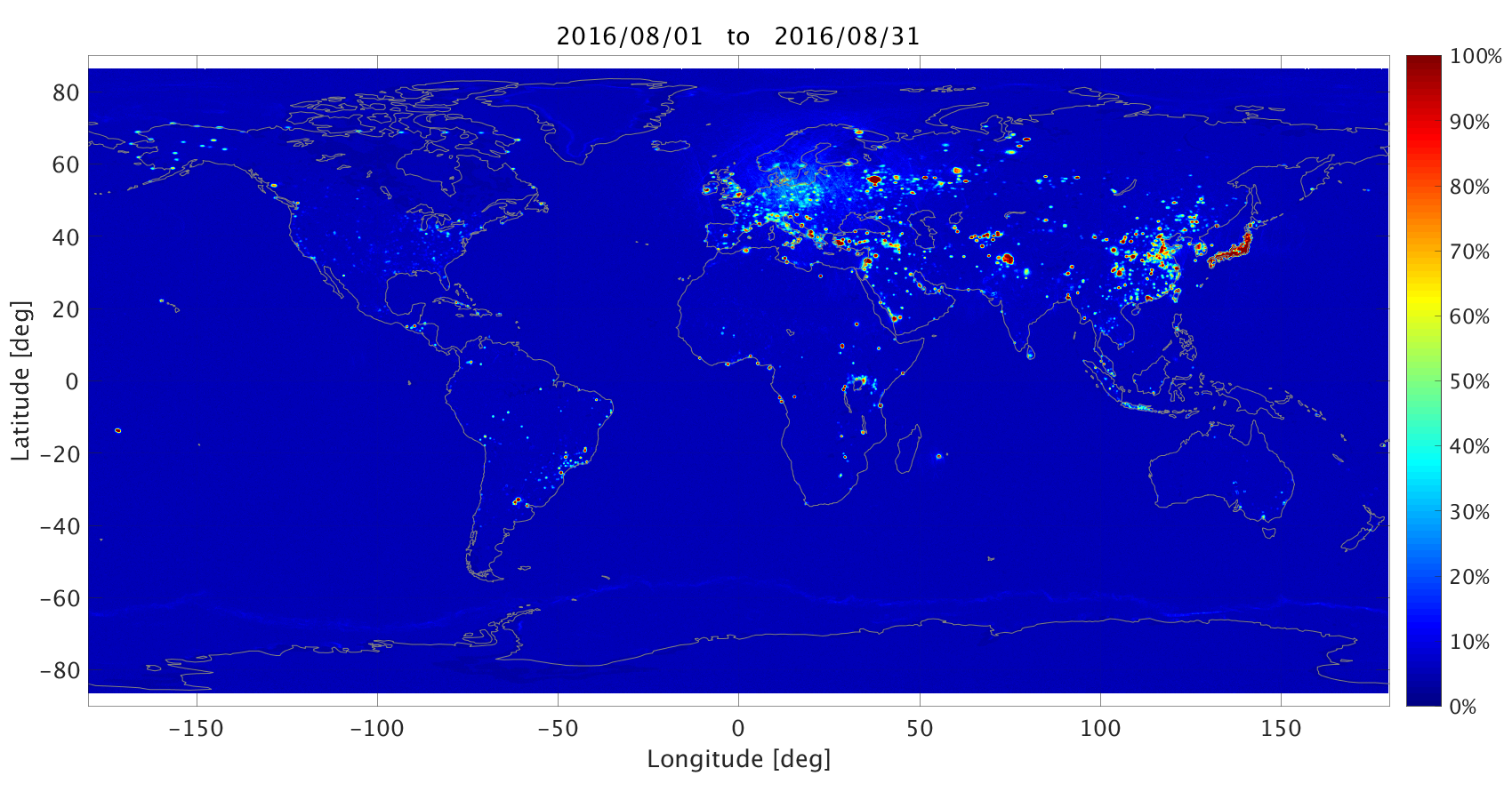
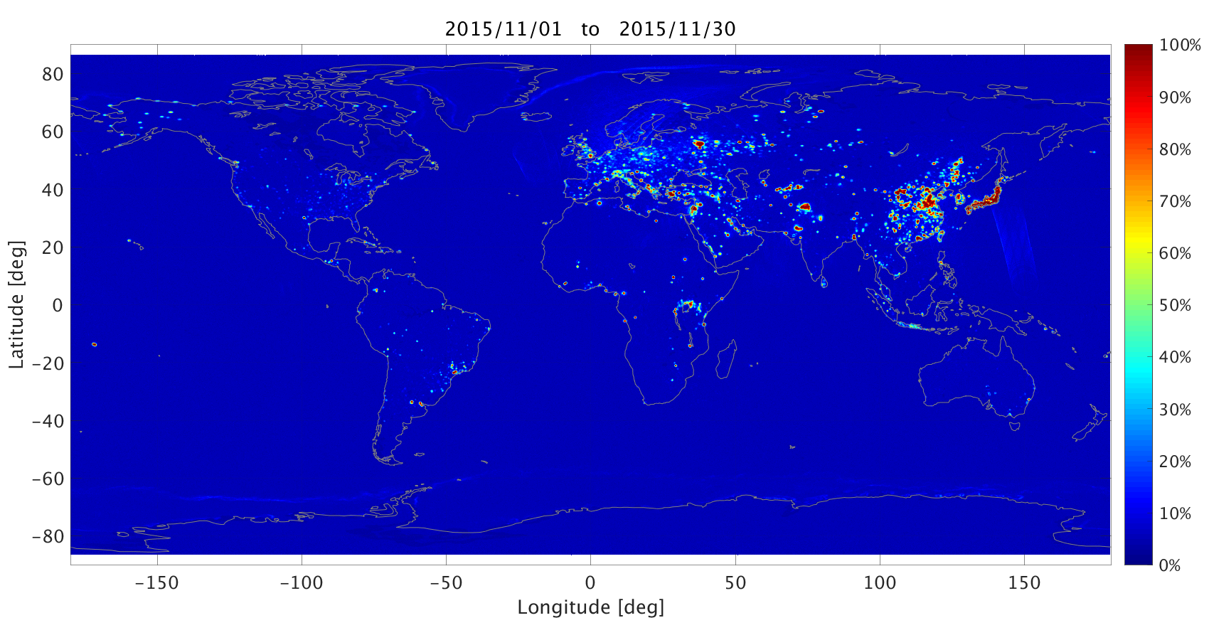
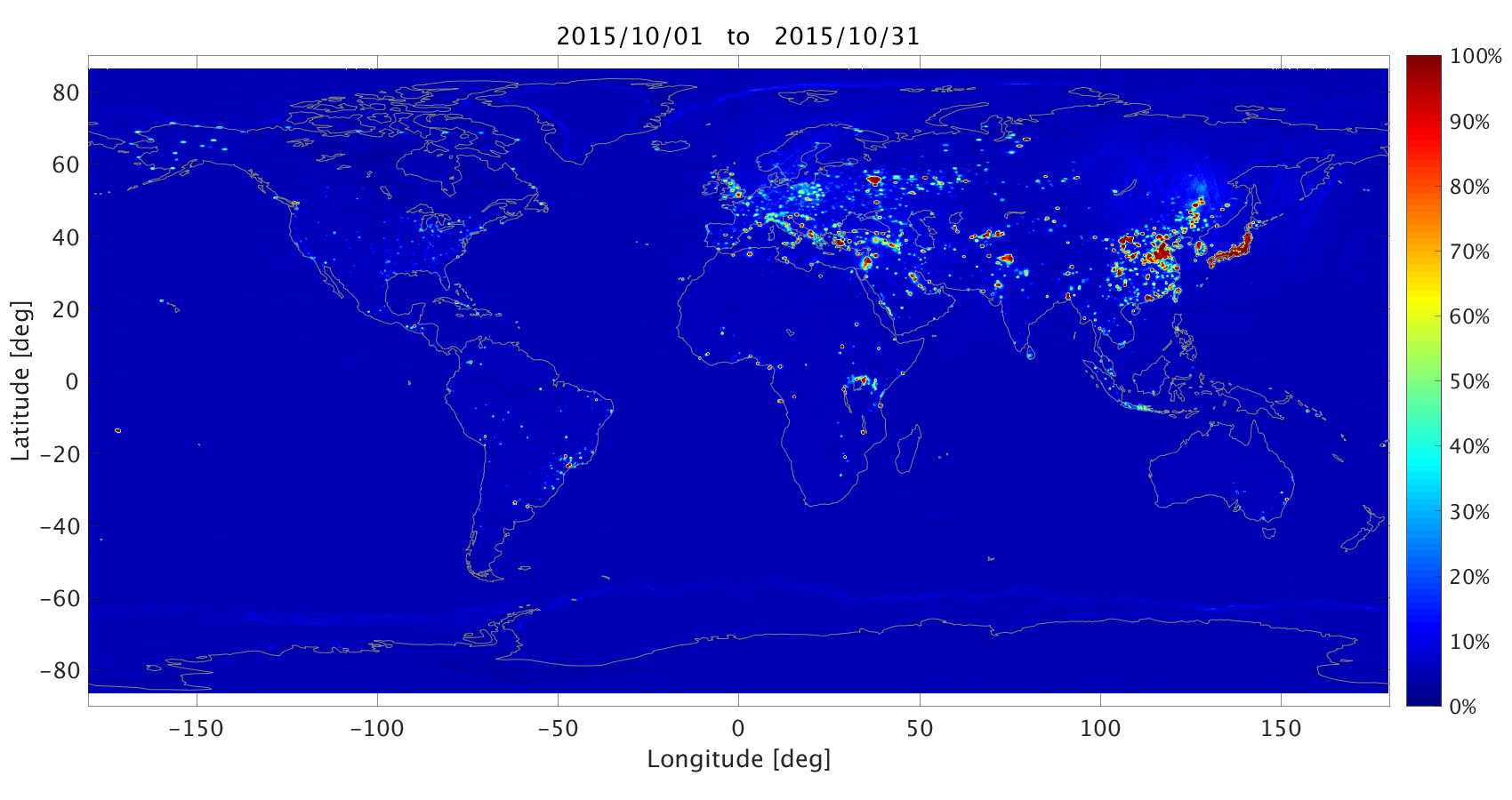
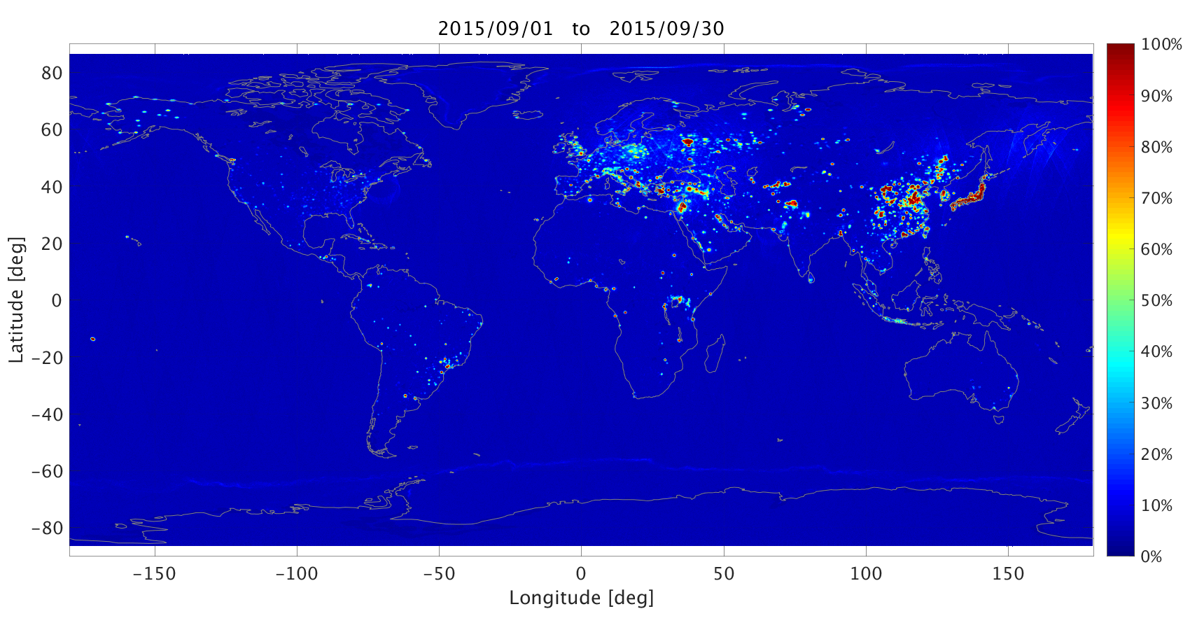
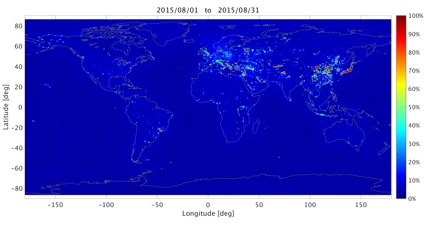
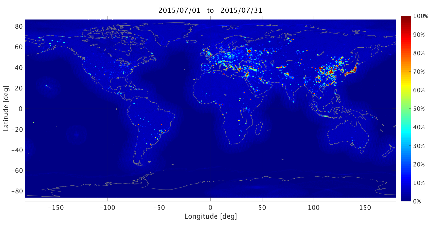
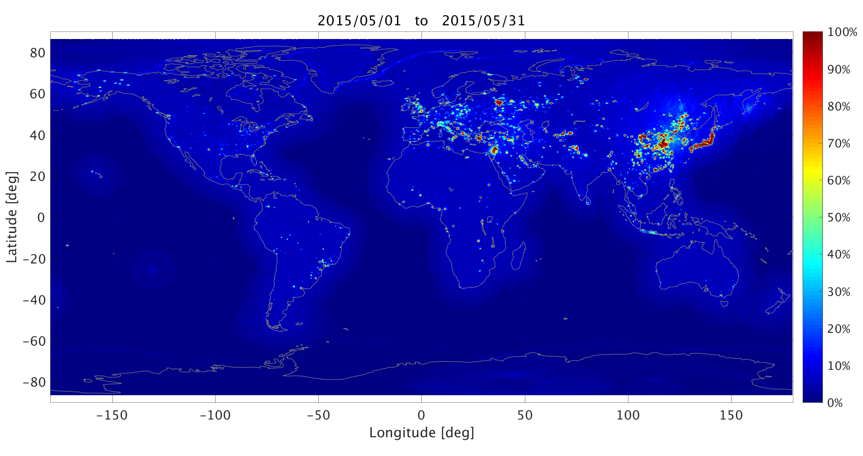
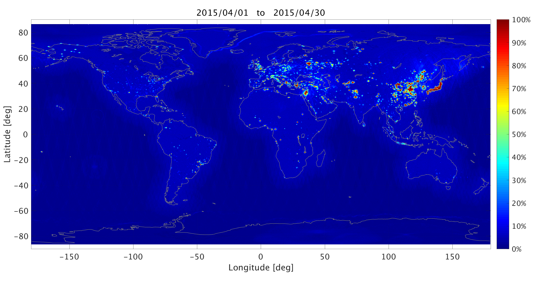
The last step in producing these maps is to average. The maps represent the fraction of RFI in each footprint as computed from the spectrogram corresponding to that footprint, averaged over all footprints whose center is within a 0.25° x 0.25° box during one month.
RFI Processing
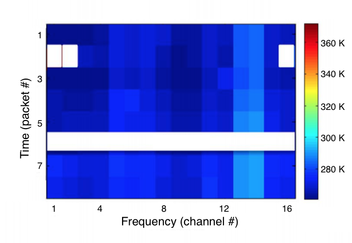
The fundamental SMAP radiometer sample is a measurement averaged over an integration time of 0.3 ms and bandwidth of 24 MHz. The measurements are produced every 0.35 ms (the extra 0.05 ms was meant to accommodate the operation of the radar, which failed shortly after launch). These data are grouped into “packets” of four samples each (1.4 ms long with 1.2ms of integration time). Four packets of science data are followed by two packets for calibration and housekeeping data. This is repeated twice to form a “footprint”, the basic unit for science data. The raw data are also available as a sequence of the 0.3 ms samples called “fullband” data, and as a function of frequency called “subband” data. In the subband data, each packet has been divided into 16 frequency channels each 1.5 MHz wide and reported as a function of time once per packet (every 1.4 ms = 8 times per footprint). For each of the fullband and subband data streams, the four modified Stokes parameters (TA,V, TA,H, TA,3 and TA,4) are generated, and kurtosis is computed for both vertical and horizontal polarization.
SMAP RFI detection algorithms are applied to both the fullband and subband data. In the case of the fullband data, an outlier-detection algorithm is used to identify pulse-like RFI and a kurtosis threshold is used to identify noise which is not random (Gaussian). The same tests are applied to the subband data and, in addition, an outlier-detection algorithm is applied looking for frequency channels where the amplitude differs from the mean. These tests are applied separately for each polarization. In addition, thresholds are applied to the third and fourth Stokes parameters, TA,3 and TA,4, and samples are marked as RFI if the thresholds are exceeded in both the fullband and subband data.
Averaging smooths the data but also raises an issue with false alarms. False alarms are inherent in the detection algorithms (i.e., selecting thresholds is a compromise between missing RFI and eliminating data). Even optimum thresholds will result in false alarms. Because there are many detection criteria for each footprint and each 0.25° x 0.25° resolution cell contains several footprints, there is always some likelihood of erroneously detecting RFI in each map grid cell. The result is a background of a low value of “false” RFI over the entire map. This can be misleading, especially over the ocean where the true level of RFI is low. To solve this problem, the maps presented on this page have the color scale set to black (no RFI) when the percentage of RFI is below 7%. With this choice (set by testing different levels), the maps highlight the true RFI and avoid the misimpression of low levels of RFI over large areas of the ocean. In addition, large changes in antenna temperature such as those occurring between land and water along coastlines can be erroneously interpreted as RFI. The RFI detection algorithm has been tuned to minimize this problem. However, the same approach cannot be used at the ever-changing boundaries between sea ice and water, which therefore appear as faint lines in the sea close to Antarctica and the Arctic Ocean.
References
Piepmeier, J.R., P. Mohammed, De Amici, G., Kim, E., Peng, J., and Ruf, C. (2016). Soil Moisture Active Passive (SMAP) Project, Algorithm Theoretical Basis Document, SMAP L1B Radiometer Brightness Temperature, Data Product: L1B_TB (Rev. B), NASA Goddard Space Flight Center, 83p.
P. de Matthaeis, D. M. LeVine, Y. Soldo and A. Llorente, "Study of a Strong L-Band RFI Source," in IEEE Journal of Selected Topics in Applied Earth Observations and Remote Sensing, vol. 14, pp. 9495-9503, 2021, doi:
10.1109/JSTARS.2021.3104264.
Click on the images (below) for a closer view.